|
This type of timebase is one of the commonest in use today. It has good linearity, a high top frequency limit, but a poor fly-back time.
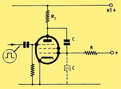
Basic circuit.
A basic form of the Miller circuit is shown above. The suppressor grid is held at a negative potential which cuts off the current in the valve. If the suppressor were caused to rise to cathode potential, current would flow and the anode voltage would drop. This drop would be transferred to the control grid via the capacitor C. If the control grid were cut off by this voltage, current would cease in the valve, and the anode would rise. The grid, therefore, drops to a negative potential just short of cut-off and current will flow in the valve.
From this point onward, one way of describing the action is to consider the 'Miller effect'. This states that the capacity between anode and grid is multiplied by the gain of the valve and appears as an imaginary capacitor between cathode and grid. The dotted capacitor Cag therefore has a value of approximately A x C where A is the gain of the valve.[1] Now the grid leak R is returned to a positive potential, so Cag begins to charge toward that potential.
The anode, therefore, falls in potential because of the positive 'movement' of the grid. The capacitor Cag will be charging non-linearly, but the change in voltage across it will be quite small, say four or five Volts. The anode, however, will fall perhaps 200 V. Such a tiny portion of the total charging excursion of Cag is actually used, however, that it is almost perfectly linear, and the anode waveform will therefore be linear also.
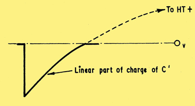
Part of grid waveform.
The diagram above shows the grid excursion considerably enlarged to show the comparative linearity of the charging curve used. When the voltage has fallen to a very low value, the valve will 'bottom'. This means that the anode voltage has fallen to a value where the grid no longer has any control over the anode voltage.
The 'run-down', as the anode voltage excursion is called, will cease and the grid will return to its normal potential, i.e., approximately at ground. If, as the instant of bottoming occurs, we cause the suppressor grid to be cut off again, the anode voltage will return to the HT voltage. Note that during the run-down, the real capacitor C has been discharging, and upon cessation of the run-down it will recharge toward HT+, through the anode load resistor R.
Normally, the load resistor R1 is large so that a high gain is obtained from the valve, and R, the charging resistor, is also large in order to avoid excessive grid current. The rate at which the anode runs down is given by: V/CR Volts/sec, where V is the potential to which the grid leak R is returned; C and R are as indicated on the circuit.
As an example, if the grid leak were returned to +250V, C were 0.01μF (0.01 x 10⁻⁶) and R 1MΩ (1 x 10⁶), the rate of the run-down would be: 250/0.01 x 1 = 25kV/sec.
If the total anode excursion were 200V then the time taken to run down would be t = 200/25,000 = 0.008 secs.
Fly-back Suppression
The fly-back time will be long because, as already mentioned, the anode load R1 must be large to obtain high gain from the valve, but C recharges through it, ready for the next run-down. In order to overcome this difficulty, it can be arranged to switch off the current in the CRT during the fly-back period.
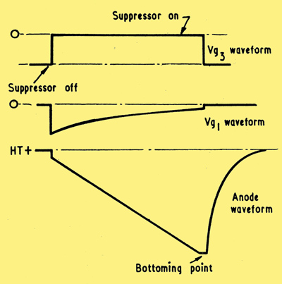
Suppressor grid waveforms.
In the diagram above the suppressor waveform is shown. This takes the form of a 'square wave', that is, a sudden change from one constant voltage to another. Now if this waveform were applied to the grid of the CRT, it would drive it positive during the run-down and current would flow. The spot on the CRT screen would, therefore, be visible. When the fly-back occurred, however, the grid would be driven negative, the current in the tube cut-off, and the spot would disappear during fly-back.
At this point, it is worth mentioning that there are two modes of timebase operation. When the circuit is operating in a freely-oscillating condition and producing a wave-form, it is said to be 'free-running'. This is suitable for observing sine waves or any waveform where the part to be observed is comparable in duration with one complete cycle. In some applications, however, one may wish to examine a short pulse of perhaps 1 microsecond, which only occurs every tenth of a second. The timebase would have to run at 10 Hz if it were free-running, in order to observe the pulse steadily on the screen. However, if the pulse only lasts 1 microsecond and the spot moves across the tube in one-tenth of a second, the pulse will be too short to be seen.
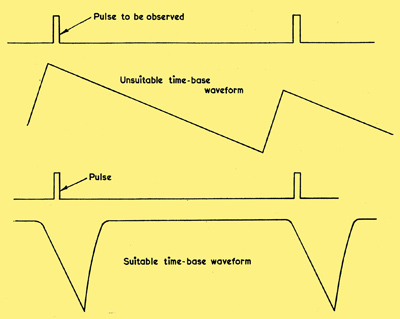
Free running and triggered waveforms.
In order to overcome this effect, a timebase may be used in the 'triggered' or 'single stroke' mode. Here the timebase is started on receipt of a 'trigger' which may be the pulse to be observed. The timebase will produce one sweep, fly back and then rest until the next pulse occurs. This mode of operation can be very useful for television work, where complex waveforms have to be examined, some of which are short compared to the time in which they occur. The lower waveform shows a typical short pulse and the timebase waveform required to enable complete examination of it.
This digression on the modes of timebase operation does not, however, explain where the square wave comes from. There are many ways of generating square waves, but for the Miller timebase a frequently used one is the transitron', which may use the same valve as the timebase itself. The combination of Miller and transitron produce a timebase oscillator with linear sweep for the tube, automatic fly-back suppression and quite good synchronising characteristics. Stig Comstedt as well as suggesting ways to make the explanation clearer has also added that the combination of Miller and transitron was known as the Phantastron. (A term new to me. Ed.) The transitron may also be used as an ordinary oscillator, a frequency divider, or even a TV sync separator.
[1] The data-sheet for the EF91 gives the Cag as less than 0.008 pF.
|