▼ Menu

    
Extras ▼

How to use Voltage Amplifier Load-lines

We have examined the last of the tree important constants of the valve, this being amplification factor, or μ. We saw also the relationship between the constants, as is given by μ = gm x r_a, gm = μ/r_a or r_a = μ/gm. We next discussed a method of finding the dynamic voltage gain of a valve under working conditions when an anode load is included in the circuit, and found that this is equal to μR_L/(R_L + r_a) where R_L is the anode load.

We shall now proceed to an alternative method of finding voltage gain under dynamic conditions.

The Load-line

A simple, and accurate, method of finding dynamic voltage gain under working conditions employs a graphical treatment applied to the published I_aV_a curves for the valve.

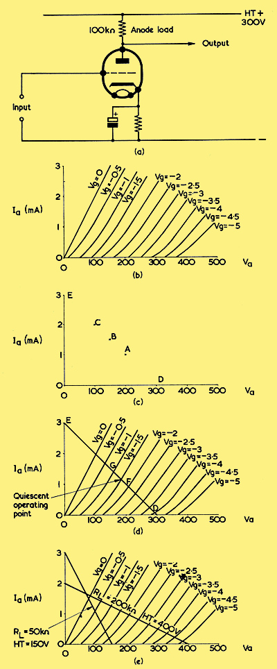
(a) A triode voltage amplifier. Cathode bias is assumed
(b) A set of I_aV_a curves, as could be given by the triode of (a)
(c) Plotting an anode voltage and anode current curve for an anode load of 100kΩ and an HT voltage of 300. The curve turns out to be a straight line
(d) Line DE, from (c), super-imposed on the I_aV_a curves of (b), provides a load-line for an anode load of 100kΩ and an HT voltage of 300
(e) load-lines may be drawn for any reasonable anode load resistance and HT voltage. Two examples are shown here

Above: (a) shows a triode voltage amplifier, and we shall assume for the purpose of explanation that its anode load has a value of 100kΩ, and that the HT voltage applied to the circuit is 300. A set of I_aV_a curves for the triode is shown in (b). When the triode passes anode current, its anode voltage must obviously be lower than that at the HT positive supply terminal because of the voltage dropped in the anode load. Indeed, it is the function of the anode load to cause a voltage to be dropped, thereby enabling an alternating voltage to appear at the anode which is an amplified version of the alternating voltage applied to the grid. Since the anode voltage depends upon the voltage dropped across the anode load resistor, it becomes possible to draw an anode current-anode voltage curve based on this single factor alone. In (c) we commence to plot such a curve, and we use the same anode voltage and anode current axes (that is, zero to 500 Volts and zero to 3 mA respectively) that we employed in (b).

We could start our work on the curve by plotting anode voltage for an anode current of 1 mA. From the Ohms Law relationship, E = IR, we know that a current of 1 mA flowing through a 100kΩ resistor causes a voltage of 100 to appear across it. Since the HT voltage is 300 this means that an anode current of 1 mA results in an anode voltage of 200, the remaining 100 Volts being dropped across the anode load resistor. The appropriate plotting point on the graph, designated A in (c), can thus be marked in. At 1.5 mA anode current there will be a voltage drop of 150 Volts across the anode load resistor, resulting in an anode voltage which is also 150. This gives us plotting point B in the diagram. An anode current of 2 mA results in a drop of 200 Volts across the anode load resistor and an anode voltage of 100. The result is shown as plotting point C.

As we continue this process it soon becomes evident that what we are actually doing is making plotting points for a straight line. The fact that the curve is a straight line is to be expected, when we consider the simple direct relationship between the voltage dropped across the anode load resistor and the anode current (E = IR), because equal changes in anode current cause equal changes in the voltage across the load and, hence, in anode voltage. Since our curve is a straight line, only two plotting points are really needed on the graph. All that is then required is to draw a straight line through these two points and the curve becomes complete. Armed with this knowledge we can, further, choose figures for the plotting points which are even simpler and quicker to find than those we have just employed. We now obtain our first plotting point by considering the case which exists when anode current is zero. If anode current is zero, the voltage dropped across the anode load resistor will also be zero, whereupon the anode voltage will become the same as the HT supply voltage. In our present example the HT voltage is 300, and we can consequently plot point D in (c). Point D corresponds to 300 Volts on the V_a axis, and to zero on the I_a axis. The next step is to find the anode current which would flow if the anode voltage were zero. (In practice, this would be the current which flowed through the anode load resistor if the anode and cathode of the valve were short-circuited together). Keeping to the figures in our present example, 300 Volts would then appear across the 100kΩ load resistor with the result that (from I = E/R) a current of 3 mA would flow. Thus, zero anode voltage corresponds to 3 mA anode current, providing us with plotting point E in (c). It will be seen, incidentally, that points D and E are directly in line with the previously obtained points A, B and C.

Let us now superimpose the information resulting from points D and E of (c), which apply to an anode load of 100kΩ and an HT voltage of 300, on to the I_aV_a curves of (b). This we do in (d). We mark our plotting point D and our plotting point E, and we then draw a straight line between them. Whatever the grid voltage of the valve (and assuming there are no components external to the circuit which may alter the effective value of the anode load) the anode voltage and anode current must lie on the line DE because of the presence of the 100kΩ anode load resistor and the 300 Volt HT supply. We can put the line DE to good use by observing the anode voltages which correspond to different grid voltages. Thus, the V_g = -2 curve cuts line DE at point F, which corresponds to 205 Volts on the V_a axis. The V_g = -1 curve cuts line DE at point G, which corresponds to 160 Volts on the V_a axis. So, with an HT voltage of 300 and an anode load of 100kΩ, a grid voltage of -2 causes the anode voltage to become 205, and a grid voltage of -1 causes the anode voltage to become 160. We also learn that a change of grid potential of 1 Volt (from -2 to -1) results in a change of anode voltage of 45 (from 205 to 160). The voltage gain with the 100kΩ anode load resistor is therefore 45.

In a practical circuit, the valve will require a fixed grid bias voltage, and a suitable value may be obtained with the aid of a graph such as that of (d). It is usual to have a grid bias voltage which causes the anode voltage to lie between about 0.4 and 0.8 of the HT supply voltage. Also, and particularly if the alternating voltage applied to the grid has a relatively high amplitude, it is desirable to ensure that the consequent changes in anode voltage are proportional to the changes in grid voltage. Otherwise, the alternating voltage at the anode will be a distorted version of that applied to the grid. Proportional changes in anode voltage will occur if there is equal spacing between the points where the I_aV_a curves of the valve cut line DE. Under the circumstances shown in (d) a grid bias voltage which would satisfy both these requirements is -1.5 Volts. This cuts the line DE at a point corresponding to about 0.6 of the HT voltage, and changes in grid voltage up to nearly 1.5 Volts in either direction cause changes in anode voltage which, by visual inspection, appear to be almost exactly proportional. So the valve, if operated with -1.5 Volts grid bias, could handle signals up to 1.5 Volts peak, and the corresponding amplified signals at the anode should be nearly identical in waveform to those at the grid.

The point where the -1.5 Volt I_aV_a curve cuts line DE signifies the conditions which exist when no signal is applied, and it is identified in (d) as the quiescent (i.e. no-signal) operating point. We find also that at the quiescent operating point the anode7current, drawn from the HT supply via the anode load, is 1.2 mA.

The line DE, which has enabled us to find out a considerable number of facts concerning the working operation of the valve, is described as a load-line. Load-lines may be conveniently drawn on any set of I_aV_a curves and their purpose is to specify the anode voltages and anode currents which exist for a particular HT voltage and a particular value of anode load resistor. To draw a load-line representing a resistive anode load, all that is required is to identify the HT voltage on the V_a axis, and to identify on the I_a axis the current which flows through the load resistor when the full HT voltage is applied across it. The line joining these two points then constitutes the load-line. To provide further illustrations, (e) shows the same set of I_aV_a curves with two more load-lines, the first of these corresponding to a 50kΩ load at 150 Volts HT, and the second to a 200kΩ load at 400 Volts HT.

The Following Grid Resistor

The load-lines of (d) and (e) enable an accurate assessment to be made of a valves performance as a voltage amplifier under working conditions and are very useful for this purpose. For approximate work involving voltage amplifiers it is reasonably adequate to work to a single anode load-line, as we have done up to now, to ascertain the performance of a valve under working conditions. However, the load-lines we have considered do not take into account the effect of components to which the output signal is applied and this factor will next be discussed.

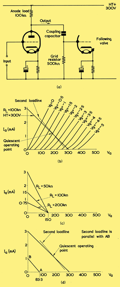
(a) In practice, a voltage amplifier will normally be followed by o coupling capacitor and grid resistor
(b) The second load-line illustrated here results from the presence of the following 500kΩ grid resistor
(c) illustrating the fact that load-line slope is proportional to load resistance
(d) A simple method of constructing the load-line of (b). Line AB has a slope corresponding to the resistance of the anode load and following grid resistor in parallel, and the second load-line CD is drawn parallel to it. To show the construction more readily, the I_aV_a curves are omitted here

It is usual for a voltage amplifier to be coupled, via a capacitor having a low reactance at the signal frequencies to be handled, to the grid of a following valve. The arrangement is shown above in (a), which shows that there is a further resistor in the circuit, this being the grid resistor of the second valve. So far as alternating voltages are concerned, this grid resistor is in parallel with the anode load of the first valve, because the coupling capacitor offers negligible reactance at the frequencies concerned and because the source of HT voltage will have negligible internal impedance. At the same time, the grid resistor will have no effect on the anode circuit of the preceding valve so far as direct voltages are concerned, because it is isolated from the preceding anode by the coupling capacitor.

To obtain a really accurate picture of the manner in which a voltage amplifier works we must, therefore, take into account any following grid resistor which appears in the circuit. The process is quite simple and we can illustrate it with an example based on the curves and load-line shown originally in (d) in the first illustration. The load-line in (b) is for an HT voltage of 300 and an anode load of 100kΩ, as occurred in (d) before, and we will assume that the subsequent grid resistor has a value of 500kΩ. The following grid resistor has no effect on the anode voltage so far as direct voltage is concerned and so it cannot affect the voltage appearing at the anode under quiescent conditions. In consequence, the 'quiescent operating point' of our original illustration (d) remains unaltered. When, however, a signal is applied to the valve, the coupling capacitor causes the following grid resistor to be effectively in parallel with the anode load resistor. To find the conditions which then hold good, we next draw a second load-line through the quiescent operating point, this second load-line having a slope which corresponds to the resistance given by the anode load and following grid resistor in parallel. This second load-line is illustrated in (b), and it defines the conditions which exist under dynamic conditions when there is a following 500kΩ grid resistor. Anode current and anode voltages will then lie along the second load-line, because the true anode load, when a signal is being handled, is given by the parallel combination of the anode load and the following grid resistor.

We have, in introducing this second load-line, had to jump a step in explanation, since we have stated that the new load-line has a certain 'slope' without describing what that 'slope' is or how it is derived. A glance at the original illustrations (d) and (e) will, however, help to explain this new concept. In (d) we have a load-line corresponding to an anode load resistor of 100kΩ, and in (e) two load-lines corresponding to loads of 50kΩ and 200kΩ respectively. It can be seen that the slope of the 50kΩ load-line is greater than the slope of the 100kΩ load-line and that the slope of the 100kΩ load-line is, in its turn, greater than that of the 200kΩ load-line. If the three load-lines were drawn for a single HT voltage, say 150, we would have the result shown in our second (c). The reason for the different slopes then becomes readily apparent. The left hand plotting point for the 50kΩ load-line, along the I_a axis, is 3 mA, the left hand plotting point for the 100kΩ load-line is 1.5 mA, and the left hand plotting point for the 200kΩ load-line is 0.75 mA. If we were to move the right hand plotting point of any of the load-lines to a higher HT voltage along the V_a axis, its slope would still remain the same because its left hand plotting point on the I_a axis moves up to compensate. The slope of the load-line is, therefore, a measure of the resistance of the anode lead.

A simple construction can be used to draw our second load-line of (b). We could start by initially drawing a line corresponding to the slope of the parallel combination of the anode load and following grid resistor. In our example, these components have values of 100kΩ and 500kΩ respectively, with the result that, from the expression for two parallel resistors, R₁R₂/(R₁ + R₂), their parallel combination gives us a value of 500 x 100 / (500 + 100) kΩ, which is equal to 83.3kΩ. A convenient right hand plotting point for a line having a slope corresponding to 83.3kΩ would be 83.3 Volts on the V_a axis, as is given by point A in (d). Such a point is convenient because it enables our left hand plotting point along the I_a axis to be (from I = E/R) 83.3/83.3 mA and saves us the both of dividing by an 'awkward' figure for R! The left hand plotting point, B in (d), then becomes 1 mA.

We now have a line, AB, whose slope corresponds to a resistance of 83.3kΩ. All we finally have to do is to draw a line parallel to it through the quiescent operating point to obtain the second load-line. This is done in (d), in which the second load-line is the same as that of (b). The second load-line defines the anode voltage and anode current conditions for the triode of our second circuit (a), when it has an HT voltage of 300, an anode load of 100kΩ and a following grid resistor of 500kΩ and it is referred to as the dynamic load-line for these conditions. (In (d) the 1_aV_a curves of (b) are omitted to enable the load-line construction to be shown more clearly).

The load-lines and load-line construction we have described in this article apply to voltage amplifiers having resistive anode loads and whose output is coupled to following grid resistors. We have used numerical examples to illustrate the manner in which the load-lines may be drawn, but it will be apparent that the principles involved can be applied to any reasonable values of anode load and subsequent grid resistor. In general, the procedure to be adopted consists of drawing the anode load-line, as dictated by the HT voltage and the resistance of the anode load, and of then finding the quiescent operating point which sets the optimum value for grid bias. To obtain a complete picture of valve performance, the dynamic load-line, whose slope corresponds to the parallel combination of anode load and following grid resistor, is then drawn through the quiescent operating point. Frequently, the following grid resistor will have a value which is three or more times greater than that of the anode load, and the dynamic load-line will not indicate results which are very different from those indicated by the anode load-line. On the other hand it can also happen that the points where the I_aV_a curves cut the dynamic load-line are not as equally spaced as occur with the original anode load-line. It may be desirable, then, to alter the values of the circuit components or the position of the quiescent operating point to obtain best results as prescribed by the dynamic load-line. If the quiescent operating point is moved, its new position will then correspond to a new value of grid bias for the particular voltage amplifier under consideration.

In the next article we shall pass on to the characteristics of practical triode valves.

Return to series contents, or to amplification factor and dynamic voltage gain or forward to practical voltage amplifiers.