|
To get a proper understanding of what a valve is doing and to know when it is being used efficiently, it is essential to understand how to read valve load diagrams. Unfortunately, on the incorrect assumption that it is a complicated business, many people shirk trying to understand them. The purpose of this article is to explain both the preparation and use of these diagrams in the simplest possible manner.
Valve curves, like guardsmen's uniforms, are divisible into two classes the ones to be looked at and the ones to be used. Those printed on the slips accompanying the valves and in the less detailed catalogues are usually of the former class and are fairly easy to understand, though it is of relatively little importance whether they are understood or not, for they give only very general information - not even enough to distinguish a pentode from a triode. They are of the type which show scales of anode current and grid voltage, with a separate curve for each anode voltage.
The other sort look very much the same except that anode and grid voltage have changed places. They can be used to disclose a great deal of useful information about the valve to which they refer, but as it is necessary to add a number of mysterious curves and straight lines, many readers no doubt prefer to do without the information rather than wrestle with the intricacies of the diagram.
This is a pity, because it is really quite easy to master the valve load diagram, as it is called, and thereafter form a very clear mental picture of what a valve is doing, and whether it is doing it properly. In particular, one is able to compare for oneself the merits of different types of valves, with three, four, five or more electrodes, that are offered for any particular job.
The apparent difficulty probably consists of the representation of current, voltage, resistance and power all at once on a single diagram. This would indeed be confusing if these were all separate and independent quantities, for it would involve four dimensions, a condition popularly associated with the occult. But there are really only two dimensions - current and voltage - and they can be represented as height and breadth on a piece of paper. The other two quantities are combinations of the first two. Power is current multiplied by voltage, and as height multiplied by breadth is area, power appears as area on the diagram. That seems quite sensible. Then resistance, according to friend Ohm, is voltage divided by current. That may appear less easy to show on the diagram, unless one remembers that a gradient of, say, one in four, is represented by the fraction ¼. So it is reasonable to suppose that one divided by four can be represented as a gradient. A resistance of 1,000 Ω, or one Volt divided by one milliamp, is represented by a line sloping one milliamp division up for every Volt division along.
Anode Volts - Anode Current
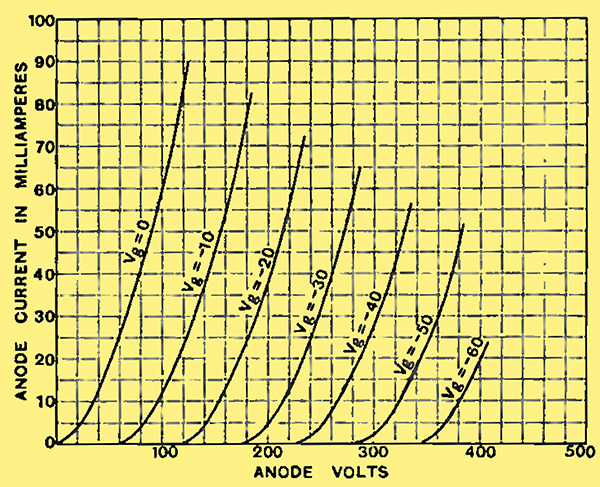
Fig. 1.- Typical set of anode volts/anode current curves for a triode valve.
Now, looking at Fig. 1, which is a typical set of curves for a triode power valve, the anode voltage and anode current scales are shown extending horizontally and vertically. The lines sloping upwards to the right represent the behaviour of the valve. The one marked Vg = 0 was obtained by making the grid bias equal to 0 and gradually increasing the anode voltage, noting.the corresponding current. The height of any point on the curve was made to mark the current at the voltage represented by the distance to the right. The same was then repeated with a grid bias of 10 Volts, giving a very similar line shifted to the right, and so on for other bias voltages. There could be, of course, an infinite number of such lines, but one can imagine the intermediate ones fairly easily.
According to what has just been explained, if another valve's lines sloped more steeply it would show that that valve had a lower anode resistance. The other resistance that enters into the combination in order to obtain a useful result is the resistance of the load, which may be a loud speaker. This resistance is distinguished by sloping up to the left, but at the moment we don't know where to put it. First of all certain areas must be declared out of bounds, as in Fig. 2.
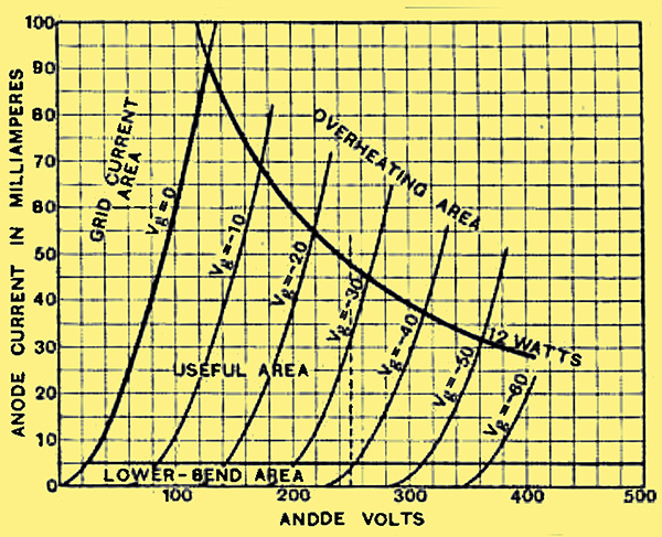
Fig. 2. - Areas that must be ruled out of bounds through various causes.
All the space to the left of the Vg = 0 line corresponds to positive grid voltage which with ordinary valves results in great current and distortion so that area is forbidden. Then the valve curves must reasonably straight and evenly distributed or another form of distortion is caused. This requirement cuts out the strip close to the voltage scale, just how much is cut out will be seen later. The this boundary is laid down by the maximum amount of power that the valve can deliver without overheating, and is usually approached only in an output stage, in the particular valve illustrated the limit is 12 Watts. A power of 12 Watts is represented by a rectangular area having two of its sides formed by the Volt and milliamp scales, and the other two chosen to enclose the right amount of space. For instance, 250 Volts and 48 milliamps multiply up to give 12,000 milliwatts, or 12 Watts, so that is one area that fulfils the conditions. But it is better not to trouble marking off its four sides, because there are endless numbers of other areas that also represent 12 Watts, and it is enough simply to put a dot at the top right-hand corner. If the same is done for a number of other pairs of numbers such as 120 and 100, and 300 and 40, and the dots are joined up, a curved line is produced and may be marked 12 Watts. The line itself does not represent 12 watts; it indicates that any rectangular area which does not poke above it is within the 12 Watt limit.
Having thus laid out the pitch, we are free to move within it. A starting point must be chosen, by selecting the right anode voltage and grid bias, such that the fluctuations of current and voltage that take place when the valve is working can be represented by a line, the load line, extending each side of it. The object preferably is to get the most out of the valve, and is represented by making the line as large as possible. The importance of the boundaries begins to appear at this stage. We have seen that the slope of, the load line represents its resistance. a in a sense its length represents the output power which is actually delivered to the load, because, being a sloping line. it may he looked on as the diagonal of a rectangular area, and area is power on the diagram (Fig. 3). So, to find the output power, complete the rectangle, either with a pencil or with the eye, and divide the area by 8. [★] The vertical side of the rectangle represents the current swing or twice the peak current, or 2√2 times the RMS current. Similarly for voltage. So the power output, which is RMS current multiplied by RMS voltage, is equal to current swing × voltage swing = 2√2 × 2√2. Area of rectangle around load line/8.
Drawing the Load Line
The line must not he drawn just anywhere ; there are definite rules. The starting point, to which the valve is adjusted by bias or HT, must be at the centre or very near it. Then next, the load line must cross as many grid volt lines on one side of the initial point as on the other. Thus, if the initial point is at a bias of -30, and it extends to 0 on the one side it must go to -60 on the other; and if it cannot do this and still keeps the initial point within 5%. of its centre, it is disallowed. It is this requirement that calls into existence the boundary at the foot, where the grid voltage lines crowd up together and if used would make the two halves of the load line flagrantly unequal.
The zero-bias boundary must also be strictly respected, and the 12 Watt line must not be passed by the fixed initial point, because it would be caught out by the excessive rise in temperature. This rise is fairly slow to act, however, and the working point, whose excursions trace out the load line, is able to cross into forbidden territory because it does so only for a fraction of a second and then it is back again before the temperature has time to realise that anything is wrong.
Maximum Power Output
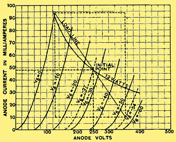
Fig. 3.- Adding the load line and completing the power rectangles.
Suppose we take the field and go all out for the full 12 Watts that can he put into this particular valve without causing it to get unduly heated. Any point on the 12 Watt line represents an adjustment that would cause the valve to draw 12 Watts from the supply, but generally the anode voltage is restricted either by the makers' advice or by convenience, and in this valve is taken to be 250. Running upwards from the 250 Volt mark to meet the 12 Watt line (Fig. 3), the initial point is fixed, and so is the grid bias, which is between b 25 and -30; call it b 27. And of course the anode current is likewise fixed, at 48 milliamps.
The load line can be drawn to the left until it hits the boundary, in which case it has traversed 27 grid Volts. So according to the rules it must go 27 Volts in the other direction, to -54.
If the load line is made very steep, almost vertical, it can go a long way up, but only a much shorter distance down, and that breaks the rule which requires the starting point to be within 5% of the true centre. So to make that right it would be necessary to shorten the line at both ends, which is not at all what is wanted. If the line is made nearly horizontal, that is to say, if the loud speaker or other load is very high in resistance, the previous difficulty is avoided, but the area drawn with the line as diagonal is very small. So it is best to choose an intermediate position, like that shown, which makes the initial point come roughly half way between the two boundaries.
Two dotted rectangles are shown; the one drawn round the load line has an area that represents eight times the useful power put into the load by the valve. The other represents the power put into the valve. If the valve were a perfect device it would give as much as it got, and these would be equal; the load area would be eight times as great as the other one. But the two areas are much more likely to be nearly equal, - or at most in the ratio of 2 to 1. So that most of the power put into the valve is wasted.
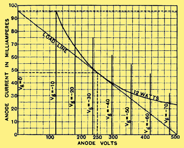
Fig. 4. - An unattainable ideal; the load diagram for a perfect valve.
Looking about, as we all must be in these days, for causes of waste, we see that if the left-hand boundary were removed the load-line area could expand without affecting the input power area. To make the boundary disappear the valve curves would have to be vertical, and as a vertical line means zero resistance, it is the same thing as saying that the valve would have to have no AC resistance. This is not practicable, but Fig. 4 shows what the diagram for a perfect valve would look like. It is quite obvious that the load-line area is four times as great as the input power area, so the output is half as great as the input. Thus the maximum efficiency even of a perfect valve is only 50%, provided there is no distortion.
DC Dissipation and AC Output

Fig. 5. - Load diagram of a valve with an efficiency of over 50%.
The last stipulation is important, because if the valve is operated where the lines crowd up at one end, so as to cause severe distortion, the efficiency is improved.
In Fig. 5, where this effect is represented, it is obvious that the large dotted rectangle around the load line is more than four times the size of the small rectangle in the lower left-hand corner, and therefore the output is more than 50% of the input. To take an extreme case, if one half of the wave is cut off entirely, so that it must be supplied by another valve, as in the QPP system, the theoretical maximum efficiency is π/4 otherwise 3.14/4,or nearly 80% That is an advantage entirely in addition to the primary object of the system, which is to restrict the current to that actually required at any moment, and so avoid letting it run to waste during intervals and quiet passages. Therefore, even when working at full power there is a substantial saving.
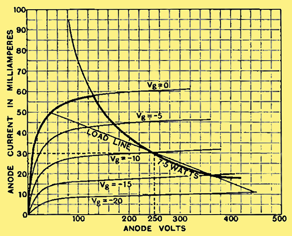
Fig. 6. -Showing why a pentode is inherently more efficient than a triode.
Fig. 3 has shown the rather poor actual efficiency of a triode valve, and Fig. 4 the maximum in an ideal theoretical valve. There is, however, a better approximation to the latter than the triode, and Fig. 6 shows how the peculiar shape of the pentode curves pushes back one of the boundaries and gives more room for fitting in a large load line. The anode voltage can swing right down to about 40, whereas the triode of Fig. 3 wastes the first 130 Volts. A triode cannot in real life do much better than 20%, but a pentode can do 30%, or even 40%. An efficiency of over 50% has been claimed, and this condemns itself with its own mouth, because it can be obtained with a single valve only by distortion.
Nevertheless the load diagrams make quite plain why a greater amount of sound can be obtained with a pentode than with a triode, the power supply being the same for both; or alternatively the same amount of sound for less power in the case of the pentode. They also make plain a strong point in favour of Class B amplification, employing special triodes in which the grid current restriction is abolished, and with it the lost space on the left. The overheating boundary also is virtually abolished, because at the initial point the anode current is nearly zero, and even when working 'all out' the temperature rise is not likely to be anywhere near the danger mark.
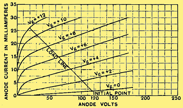
Fig. 7. - Diagram of a Class B valve, showing how nearly it approaches the theoretical ideal.
Fig. 7 shows a diagram for a Class B valve, which is a very close approach to the theoretically perfect. An actual efficiency of well over 50% is obtainable. It has the unique combination of three claims to efficiency:-
- The theoretical limit of efficiency is nearly 80%.
- Owing to the shape of the curves this limit is approached more closely than by other valves.
- The efficiency at low power is maintained by the quiescent effect.
|