|
Practical design procedure for series-valve types
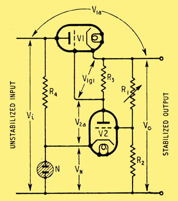
Fig. 1. Basic circuit of series-valve stabilizer, in which the output voltage Vo is adjusted by varying R1. N is the voltage reference standard, and V2 the negative feedback amplifier.
Although voltage stabilized power units have been fairly widely employed for some years, it seems that there are still many who do not fully realize how useful they are, or who have insufficient information about their working and design. As regards the first point, anyone who has once become accustomed to using a stabilized power unit will probably confirm that if is practically indispensable. As to the second, this article may be a partial answer.
At one time the need for sources of steady DC was met by secondary batteries, in spite, of their high cost and maintenance trouble, because the alternative - the rectified AC power unit had a comparatively high internal impedance and consequently bad 'regulation'. That is to say, the output voltage varied considerably with the current drawn. An additional cause of substantial voltage variations came when power stations, in order to avoid the more drastic operation of load shedding, began to practise frequency and voltage reduction. In the meantime, requirements for low ripple and noise content have become increasingly stringent. The development of stabilization technique, however, has now reached a state at which it is possible to dispense with batteries for even the most exacting requirements.
Of the several distinct methods that have been adopted, the most popular and generally useful, and the only one to be considered here, is that shown in principle in Fig. 1
The whole load current passes through V1, which is made to absorb any voltage variations, whether slow or rapid, so that the output is constant and steady. V1 may also, if required, be made to serve the additional purpose of reducing the voltage of the source to any desired level, within certain limits of adjustment.
The remainder of the circuit is designed to control the voltage drop in V1 in order to fulfil the purposes just mentioned, This it does by comparing a known fraction R2/(R1 + R2) of the output voltage (Vo) with a fixed reference voltage, usually (but not always) provided by the drop across a neon tube, N, The difference in voltage is amplified by V2 and applied as grid bias to V1 in the correct polarity to oppose any change in Vo.
The device is closely analogous to the governor of an engine, and is an example of DC negative feedback, a sort of amplified cathode follower, Obviously one of the prime objects in design is to make the voltage amplification so large that the change in Vo necessary to neutralize (via V2) any fluctuations in source voltage is negligibly small. At zero frequency the feedback is reduced by the potential divider R1 R2 but this reduction can be avoided at hum frequencies by short-circuiting R1 with a capacitor.
If the gain, reckoned from the junction of R1 and R2, is made so large that any variations in voltage across R1 needed for feedback are less than, say, 1 per cent, and the reference standard is also very constant and accurately known, the current through R1 is correspondingly constant and Vo is directly proportional (within the working limits of the valves) to R2 + R2. R1 can therefore be calibrated in volts to an accuracy equal to or better than that of a British Standard first grade voltmeter. A notable example is the Tinsley Precision DC Stabilizer, in which the reference voltage is a standard cell and the amplifier a reflecting galvanometer and photocell. Any voltage from 20 to 600 can be selected, to an accuracy of 1 in 10,000.
However great the gain, some change in output voltage is necessary to effect the stabilization; but such change can be reduced to zero or even reversed, by compensation for changes in input voltage and output current. By the use of such devices it is possible to make the power unit approximate very closely, over a wide range of working conditions, to a generator of constant zero-frequency voltage with zero internal impedance.
The practical design of stabilized power supplies on these lines was discussed in an excellent article by F L Hogg. The present writer acknowledges that what follows, is largely an extension of Mr Hogg's work.
Considering now the design of stabilized power units in detail, there is first the, question of requirements. The design problem is very much eased if only a fixed output voltage is needed, or on variable within narrow limits; and similarly if the current load is more or less constant, as it often is in built-in power sources. One has then only to provide against minor variations in load, and variations, in AC supply. The latter can, if necessary, be brought within narrower limits by one of the special transformers sold for the purpose. The residual fluctuations can then be dealt with by valves and other components working on fixed adjustments very close to optimum conditions and a very high degree of stabilization obtained without much trouble.
It will therefore be more instructive to tackle the relatively difficult case of a unit for general laboratory use, in which the output voltage is required to be variable within wide limits, and the load may be anything from zero to a stated maximum. The procedure for most other specifications should then be more or less obvious.
The design will, of course. Be influenced by whether the most important thing is to stabilize against input voltage fluctuations, or load current fluctuations, or to reduce hum and noise to a very low level, or a combination of these. They correspond respectively, in the theoretical equivalent generator, to constancy of generator voltage, smallness of generator impedance, and absence of any generator frequency appreciably above zero. The length of time over which a specified performance in these respects must be maintained is also a factor to be considered, if an accurate output voltage calibration is wanted, that is yet another.
Let us assume as an objective the best all-round performance obtainable with a reasonably simple system capable of coping with wide voltage and current ranges. Its achievement can best be illustrated by an example. Suppose the maximum output is to be 100 mA at 400 V, with the mains voltage liable to vary +4 per cent and -8 per cent from normal. The easiest and most instructive procedure is to make a voltage/load-current diagram (Fig. 2). Neglecting current through V1 other than the load current Io, point A represents maximum output, and the horizontal line through it is the working line at 400 V for all load currents down to zero, assuming perfect stabilization.
Now consider the drop in the series valve V1, it can be allowed to reach its minimum under the condition of maximum output and mains 8 per cent low, and that minimum should of course be as small as possible. The limit is imposed by the start of grid current; to be on the safe side, the minimum bias may be assumed to be -1= V. The shape of a tetrode (or pentode) characteristic gives it a low Va for a given high Ia, but there is a constant screen voltage to provide. For simplicity let us assume a triode, in which the clue to a low voltage drop is low ra. At the same time we want μ to be as high as possible in order to maximize the stabilization. There is thus no doubt that high gm is needed. The best allocation of ra and μ for a given gm will be, seen more clearly later in any particular case, but in general economy calls for a low ra. As a start, take a triode-connected Mullard EL37, which is typical of a number of similar valves. Fig. 3 shows the Ik/Va characteristics. From these, at Ik = 100 and Vg1 = -1=, Va is seen to be 140 V. This must be added to Vo max in Fig 2 to give point B, the un-stabilized voltage of the source, Vi. From the data relating to a suitable power supply, the regulation curve BC can then be drawn in. Normally it droops slightly between B and C, but a straight line is generally near enough. This line is the lowest allowable, so it relates to 92 per cent of normal mains voltage. Assuming Vi at zero current to be proportional to mains input, points D and E can be marked in at 100 per cent and 104 per cent. Lines through them, parallel to CB, represent approximately the regulation curves for normal and maximum mains.
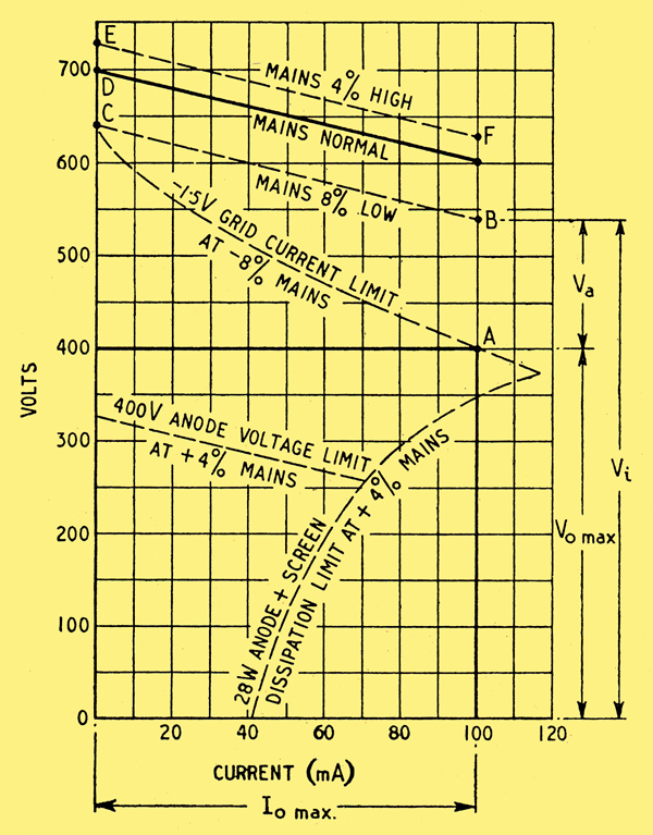
Fig.2. Voltage/current design diagram for a series-valve stabilizer.
If desired, point A can be extended into a complete curve showing the minimum drop in V1 at any load current. It is got by (so to speak) hanging the V = -1= Vg1 curve of Fig. 3 from the line CB. One could, in fact, transfer the whole family of curves from Fig. 3 to Fig. 2 but it would be rather confusing to do so for each different mains voltage.
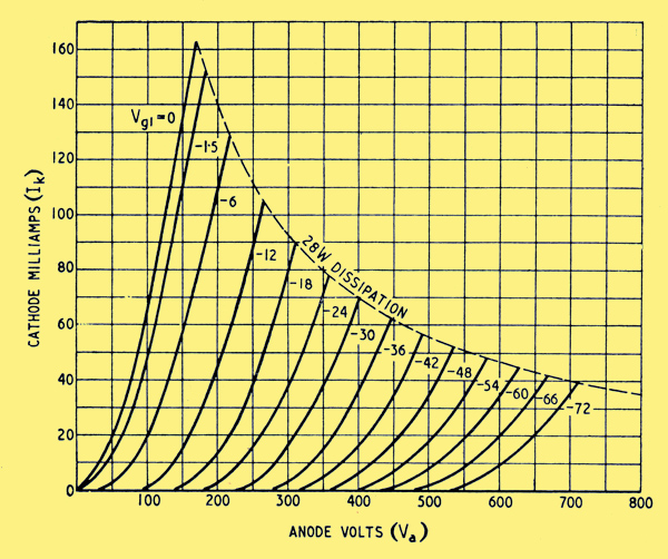
Fig. 3. Characteristic curves for triode-connected EL37 valve for V1 duty.
The most important limit is the maximum anode (actually a + g2) dissipation, in this case 28 W. It should be hung from the maximum, mains line, EF, as shown. (The vertical distance between it and EF at any point is reckoned, of course, by dividing 28 by the current in amperes at that point). The maximum rated Va; triode connected, is 400 V, and should be drawn at that distance below EF. The maximum current rating, 200 mA, is not in the picture at all.
We can now see that keeping strictly within these limits we could get any current up to 115 mA at 370 V; that at any current up to 100 mA the Vo could be varied from 350 to 400; that at a fixed output of 70 mA, stabilization against mains voltages from -8 per cent to +4 per cent is possible over a range of Vo from 260 to 450; while if Ia max were restricted to 40 mA, and the Va, + g2 limit were ignored, Vo could be varied from 0 to 500 V.
Study of this diagram should make it a simple matter to decide on a suitable power source and V1 to meet stated requirements. To obtain more than a very small range of Vo at a 100 mA rating, it is clear that a higher anode dissipation and/or lower ra is needed. One solution is to use two or more valves in parallel. This is quite feasible, but it is necessary to make sure the valves are well matched, and wise to design a little more conservatively to allow for inequality. To avoid failure of all valves if one of them goes, individual fuses, or better still a differential relay, may be worth while.
Using a pair of EL37s in parallel, making 2Ik max = 110 mA to allow for the drain in R1 R2, etc, (Ik being the cathode current per valve), and reducing the to Pa + g2 rating per valve to 26 W, we get, Fig 4.
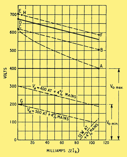
Fig. 4. Design diagram for a 200-400 V unit using two EL37's in parallel for V1.
The dissipation boundary has almost disappeared; but if one still strictly observes the Va + g2 max rating at +4 per cent mains and 2Ik min (say 10 mA) the range of Vo adjustment cannot be extended below 290 V min. To obtain a wider range, one can assume the valves will not mind the possibility of occasional breaches of this limit at low currents, or else use valves with a higher rating, such as Osram PX25 triode (500 V) or Mazda 12E1 tetrode (700 V) ; or cover the full range of Vo in steps, reducing the source voltage and R1 simultaneously with a switch.
Before going into this more closely, we should consider V2 and its appurtenances. It is clear from Fig. 1 that Vo has to be not less than the reference voltage (V N), plus the anode voltage for V2 (V2a) plus the bias for V1 (V1g1). There is therefore a practical minimum Vo with this circuit. V N is determined by the characteristics of available tubes, and in any case there are disadvantages in its being a very small fraction of Vo max, the overall feedback is reduced in the ratio Ra/(R1 + R2)and the 'error' (VN - VR2) is relatively serious. The table below gives data for some suitable tubes.
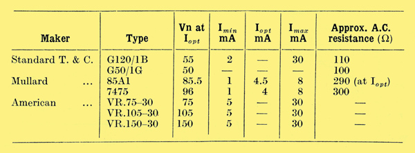
V2a cannot be reduced too far or the gain will fall off, gradually with a triode and suddenly with a pentode. As for V1g1 when Vo and Io are least it must be at its greatest. Supposing the lowest Vo to be provided is 200 V, and 2Ik min is 5 mA, this condition is represented by point G in Fig. 4, which is practically 500 V below Vi with mains 4 per cent high. From Fig. 3 the bias required is -65 V. That leaves 135 V for N and V2, which is sufficient for a tube running up to about 100 V, in series with a pentode. With G5O/1G tube Vo min can be reduced to about 125 V.
The advantage of a high μ in V1 when a wide range of Vo is wanted is now clear.
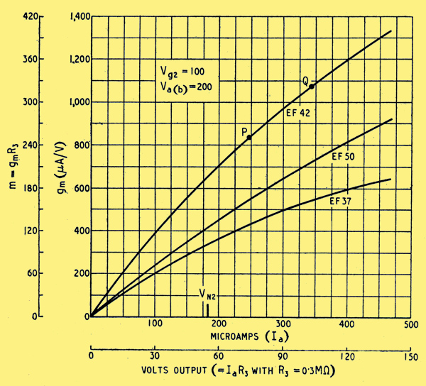
Fig. 5. Slope/anode-current or gain/output curves for three types of valve for V2 duty. VN2 is the zero V1g1 point using a G120/1B for N2.
Voltage gain (call it m) is the chief criterion for V2, and the most generally useful characteristic is a graph of gm against Ia, as in Fig. 5. Multiplying both scales by R3 converts it into a graph of approximate stage gain against output voltage. (In Fig 5 the gains shown were actually measured data, using 0.3Mω anode coupling, R3 and gm scale was derived from it on the assumption m = gm x R3) Now the required range of output voltage is known; it is from 1= to 65 V in our example. Whatever value of, R3 is chosen, Fig. 5 shows that if it is fed from the cathode of V1 as in Fig 1 the gain will vary enormously. Using an EF42 with 0.3 MΩ it ranges from about 6 at V1g1 = -l= to 230 at V1g1 = -65.
It is clear that m can be made much more nearly constant and at the same time its average level increased by feeding R3 from a more positive point. It could be fed from the anode of V1 but unfortunately the potential of that point shifts in such away that the output required from V2 when Vi varies is multiplied by μ1 + 1. Looked at another way, it is equivalent to multiplying Ri by μ1 + 1 (see Appendix c in subsequent instalment, Eqn 11b).
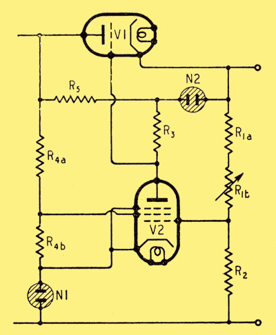
Modified feeds for V2 to ensure higher and more uniform gain.
The solution is to use another stabilizing tube, N2, as in Fig. 6. Its running voltage must be substantially less than the minimum drop across V1 (V1a) in order that the ratio of maximum to minimum drop across R5 does not exceed the working current ratio for the tube, and at the same time to ensure that the current is always less than that taken by R1 and any other permanent drains.
In our example, the limits of V1a are 105 V (A to B in Fig. 4) and 495 V (G to H). Using a G120/1B for N2, the range across R5 is thus 50 V to 440 V, and the corresponding current in R3 (if 0.3 MΩ) is 0.19 mA and 0.40 mA. Limiting the current through N2 to 4 mA say, the total maximum through R5 at 440 V is 4.4 mA, so R5 should be 100 kΩ, 2 W. The minimum current through N2 is then (50/100) - 0.19 = 0.31 mA. This is below the working range for N2, but since appreciable fluctuation of voltage across it can be tolerated that does not matter. If anything, R5 might be increased, because the current through N2 tends to impair stabilization at low Io, for it is not controlled by the feedback. It is a function of V1a and could be allowed for by a modification of Fig. 4, but normally it should not be large enough to be worth this extra complication.
The voltage across R2 is equal to that across N1 less V2g1. VN1 is (we hope) constant, and V2g1 ought not to vary much if the unit is doing its job. Its mean value may be difficult to find, since valve makers rarely show the working region below 0.5 mA very clearly; so unless one plots this part oneself it may be a case of making as good an estimate as possible. With V2g2 about 80-100 V, V2g1 averages -1.5 V for the EF42 and -3 V for the EF36 or EF37. Using an 85A1 and EF42 therefore makes VR2 84 V. The value of R2 can then be chosen to, pass a suitable current, say 5 mA: The exact value is more conveniently related to R1, however, because part of it (R1b) is the voltage control and may have to be a value that is available. Stability of R1R2 is most essential, and good wire-wound components must be used throughout. The range of voltage control in our example is 200 V, so if a 55 kΩ rheostat is used the current is 4 mA. R2 must then be (84/4) = 21 kΩ, and R1a (which must drop 200-84 = 116 V) is 29 kΩ. Maximum total 100 kΩ at 4 mA, 400 V, which is the designed maximum, so correct.
With 2I1k as low as 4 mA, R5 ought definitely to be raised, say to 150 kΩ to ensure that IN2 is always less.
The extreme range of V2g1 can be deduced from Fig. 5. The mean gain in our example, using EF42, is about 280; so a range of 63.5 V output necessitates about 0.23 V at the grid, which is ±0.136 per cent of the 84 V across R2 and therefore the same percentage of Vo. This can be analysed with the aid of Figs. 4 and 3 into the variations due to mains fluctuations and to load current. For example, at 300 V output with normal mains, change of load from zero to 100 mA (neglecting IR1-IN2) necessitates a change in V1g1 from -48 V to -19 V, represented by P to Q in Fig. 5. Dividing the voltage change, 29, by the mean gain, 290, gives 0.1 V as the change in 84 V, and so 0.36 V in 300, corresponding to a mean internal resistance of 0.36/0.1 = 3.6 Ω. The value varies considerably over the range of Io, owing to variation in I1a, being higher when Io is small and vice versa.
Similarly the Vo variation corresponding to ±4 per cent mains variation from normal at 300 V 100 mA output can be shown to be ±0.0143 per cent, or a stabilization ratio of 280:1.
Formulae for these parameters will be derived in the Appendix.
In the above calculations it is assumed that I2a is not appreciably affected by variations in the potential of any electrode other than g1. The gain m is reckoned on this basis. Reasonable, constancy of anode feed voltage has been ensured by N2. But what about the cathode and g2? It seems to be generally assumed by writers on the subject that N1 keeps the cathode steady against any variations in the voltage of the source feeding it. That is by no means true. The AC resistance of N1 at its optimum current is usually of the order of 300 Ω and it is possible for the voltage drop to vary sufficiently to upset completely the performance calculated as above. Even though the feed resistance R4 may be, say, 500 times as great, so that source variations are reduced in the ratio 501:1, it must be remembered that they are then multiplied by the total feedback gain, μm, which may be of the order of 2500.
So to preserve the stabilization it is desirable (and to use N1 as a voltage standard it is essential) to feed N1 from a stabilized source. If Vo is fixed, it is the obvious source. Keeping the current constant in this way, the best use can be made of a good tube. The makers of the 85A1 claim that its short-term stability is within ±0.1 per cent, and long-term stability ±0.2 per cent, so that it can be used as an accurate voltage standard. For this purpose it is desirable to use a circuit in which VN1 is applied to the grid of a valve, to avoid current changes in N1 via the valve; but for power supply purposes such, changes are generally negligible.
If IN1 is kept constant in this way, g2 can be tapped off the feed resistance, R4, at about 100 V. R4 itself is chosen to pass about 4 mA, compared with which I2a and I2g2 are small.
The same arrangement will do if Vo is variable over a moderate range, but it may then be desirable to substitute a regulator tube for R4b the part of R4 between g2 and k.
For a wide range of Vo control it would be necessary to gang R4a with R1b which would be rather a nuisance. It is therefore usual in a unit such as we are considering to feed N1 from the anode side of V1. Here the range of voltage variation is relatively small, but, unlike the variations of Vo; which occur only while it is being adjusted, they are 'stabilization' variations, in opposition to those provided by V2. It will be shown in the Appendix (Eqn. 10a) that the effect is as if the source resistance, Ri, were increased by a factor equal to the total gain round the loop R4N1 V2 V1, that is to say μ1mVN1/R4, which may mean a several-fold increase in apparent Ri and a corresponding loss in stabilization.
A very convenient way out of this trouble is to adjust the resistance across which V2g2 is obtained (R4b) so that its variations neutralize those in VN1. Neglecting the I2g2 variations, the correct value of R4b is thus μ2g2VN1 where μ2g2 is the amplification factor between g1 and g2 in V2. In the EF42 it is 85; but since I2g2 variations add to those in N1 the result is as if it were somewhat lower, in a measured example about 65. The value of R4b to fulfil this requirement is not necessarily suitable as regards the standing V2g2; but in our case it is, for with VN1 at 300 Ω, effective μ2g2 say 65, and IR4b at 4 mA, we have 78 V, which is quite, a satisfactory screen voltage.
Having neutralized the apparent extra Ri in this way, one may well ask why the real Ri should not be neutralized too. As the Appendix will show (Eqn. 9a), this operation is equivalent to neutralizing an added resistance in N1 equal to R4/μ1m. In our example, the mean Vi is about 600 V (Fig. 4); less VN1 this is 515 V, so, to pass 4 mA, R4 should be about 130 kΩ. Taking μ1m as 2000, the extra R4b required is 4.2 kΩ.
When R4b is correctly adjusted, then, the unit behaves as if Ri were zero; and, what is more, stabilization as regards variations in mains voltage is theoretically perfect. It is accomplished solely via the screen grid of V2, output feedback via the control grid being unnecessary, and variations in Vo nil. In practice it does not work out quite like that, because certain of the factors, notably m, are not constant. The slightest departure from exact adjustment; of R4b would, if there were no output feedback, make the stabilization fall right off. The designer should therefore, aim at the greatest possible basic stabilization by output feedback, which does not depend on critical adjustments; and then any unavoidable variations in the further improvement conferred by input feedback will be of minor importance.
For this reason it is not altogether recommended that input feedback be used to neutralize the large apparent increase in source resistance that would be produced if R3 were fed from the input side of V1, although it could do so, and would save N2 and R5 and the uncontrolled current around V1.
By increasing R4b beyond that necessary to neutralize Ri it can be made to neutralize V1a also, with the result that Ro (the resistance of the unit as a whole) is zero, and the output voltage is subject to variations in m and V1a entirely unaffected by changes in load current. At this setting of R4b the unit is somewhat over compensated for mains fluctuations. In practice one would adjust R4b to give a compromise depending on the relative importance of mains voltage and load current changes. It is practicable in this way to improve on the basic stabilization in both respects.
Part 2
|