|
- The First Triode
- The AEI Mazda Valve P61
- What Happens Inside a Triode?
- What is a Potentiometer
- Plotting the Characteristics
- Interpretation of the Curves
- Space Charge
- Saturation
- Valve Parameters (ra, gm and μ)
- ra
- gm
- μ (pronounced mu)
- The Triode as an Amplifier
- Class A Amplification
- Distortion
- Power Output
- Load Line
- Class 'B' Amplification
- Push-Pull Amplification
- Class 'C' Amplification
- Grid Current Rectification
- Anode Bend Rectification
- The Triode as an Oscillator
At the same time as Fleming was developing the two electrode valve in this country, Dr Lee de Forest was carrying out experiments in America with a view to developing a new system of wireless telegraphy.
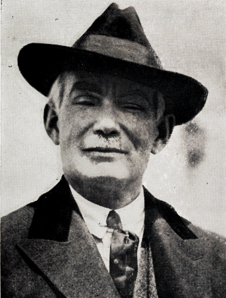
Dr Lee de Forest
De Forest noticed, in 1900, that when an induction coil was in operation the gaslight in his room diminished. This, he suggested, was due to an electrification and consequent expansion of the gases in the flame. Hence, he argued, a detector for transmitted impulses might consist of a volume of gas provided with a sensitive indicator of pressure. In 1903 he began to search for genuine response to electrical vibrations in the gas flame and, in 1905, stated that positive electricity passed through a Bunsen flame more readily in one direction than the other. In other words the flame acted as a valve. Next year he developed a partially exhausted bulb containing two electrodes, one of which was the filament of an ordinary electric lamp, the other a disc of platinum. The filament was to heat the gas between it and the other electrode. This device, he claimed, acted as a relay rather than a rectifier, such as Fleming's already established diode.
The most important development came, however, when he found he was able to influence the flow of current between the electrodes by means of an external electrode involving no metallic connections with the other electrodes. High Frequency current was passed, from an aerial, through a coil surrounding the whole bulb, and due, he reasoned, to the magnetic field produced, affected the inter-electrode current. Similarly, he deduced, comparable control by High Frequency potentials on external plates was due to the resultant electrostatic field.
This resulted, in 1906, in his introducing into the diode a second plate fixed at right-angles and adjacent to the two original electrodes. This he again connected to his aerial and the electrostatic field so produced was thus used to control the Anode Current of the system.
From this he took, in 1907, what must now seem the obvious step of placing this electrode directly between Cathode and Anode. Since, if this electrode were a solid plate, all flow between Cathode and Anode would be prevented and since his chief object was to place an electrostatic field between Cathode and Anode, this third electrode assumed the form of a wire Grid. Thus, simultaneously, the electrostatic field was introduced whilst still leaving a relatively clear path between Cathode and Anode.
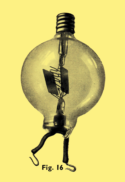
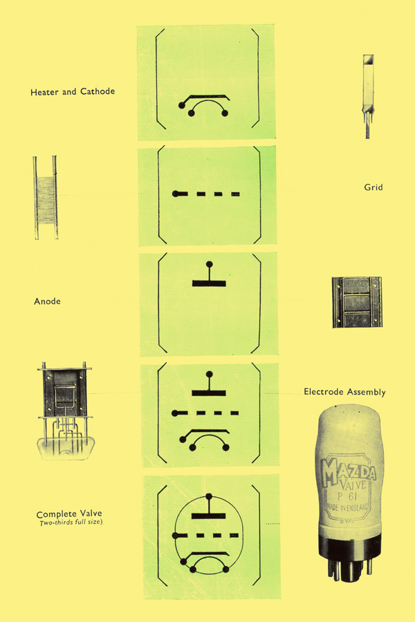
This new valve (Fig. 16) became known as the three electrode Audion, the name being derived from the Latin Audire (to hear) and the Greek Ienai (to go). Hence Audion is a device to enable us to hear electricity in motion.
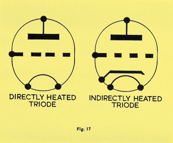
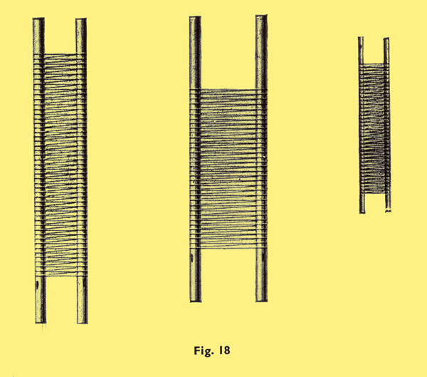
Subsequently, however, such a valve has become known as a Triode, that is having three electrodes. Cathode, Grid and Anode. It is represented, diagrammatically, as shown in Fig. 17. A selection of modern grids is shown in the enlarged photographs in Fig. 18.
In Electrons in Diodes Fig. 4 indicated the flow of electrons from Cathode to Anode. Merely introducing the Grid (Fig. 19) will have negligible effect on the electron stream, although the few electrons which actually strike the Grid may be returned to the Cathode.
If, however, the Grid is made slightly negative with respect to the Cathode (Fig. 20) some of the electrons will, each having a negative charge, be repelled and forced to return to the Cathode. The number of electrons reaching the Anode will, therefore, be less; in other words the Anode Current will be reduced.
Ultimately (Fig. 21), by making the Grid even more negative, a stage is reached when all the electrons from the Cathode are halted by the Potential and forced to return to the Cathode. The Grid acts as a tap to cut off the current, in fact this stage is known as Cut-Off.
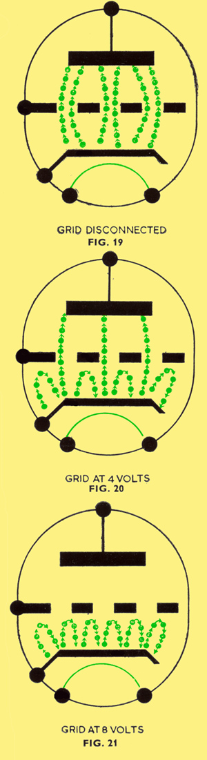
Since the Grid is physically nearer the Cathode than is the Anode it is self-evident that a change in its potential will have a much greater effect on the Anode Current than will a similar change in the Anode Potential. The Grid Potential then, may be used to control the Anode Current.
Before going any further it might be helpful to answer this question. If a length of wire A-B is connected to a battery, as shown in Fig. 22a, it is obvious that since A is joined to the positive terminal it will be at a higher potential than B. It is possible to represent this state of affairs graphically (Fig. 22b). The base line can represent the length of A-B and the height above this base line the potential above B. Hence the potential at A will be at a height P representative of the full battery voltage, whilst at Bit will be at point Q, that is, zero.
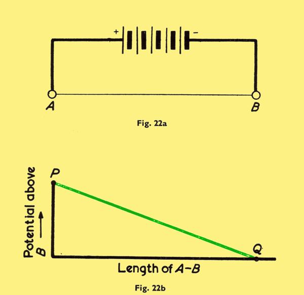
Assuming the wire A - B to be perfectly uniform along its length it is easy to see that the potential difference between any point on A - B and the point B itself will become smaller and smaller the nearer it is to B. In other words, there is an even potential drop along the length of the wire and this can be represented by the straight line joining P and Q. The height of this line at any point above the base line will represent the difference between the potential of that point and that of B.
Thus, by having a sliding contact on A-B any desired potential with respect to B (up to the maximum potential of the battery) can be selected and read on a voltmeter.
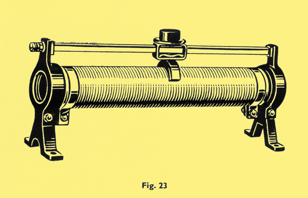
Obviously the wire need not necessarily be held out straight, it could be wound round a former (Fig. 23). Such a device is called a potentiometer and is represented diagrammatically as shown in Fig. 24.
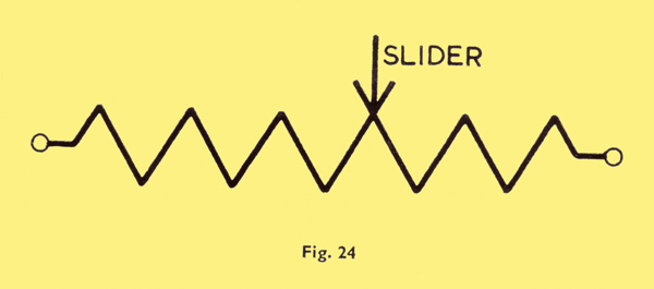
Fig. 25 shows an indirectly heated Triode, the heater of which is connected to an external source.
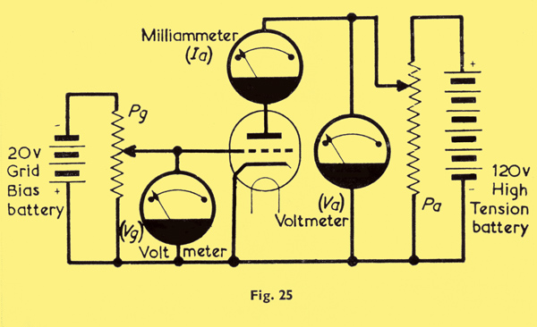
A Grid Bias Battery has its positive terminal connected to the Cathode. Across the battery is a Potentiometer Pg from which a potential negative to the Cathode may be selected by the slider and applied to the Grid. By merely reversing the battery connections a potential positive to the Cathode may be applied to the Grid. The value of this Grid Potential may be read on the Voltmeter Vg.
Similarly a potentiometer Pa across the High Tension Battery enables a potential positive to the Cathode to be selected and applied to the Anode, its actual value being given on the voltmeter Va. Anode Current is read on the Milliammeter la.
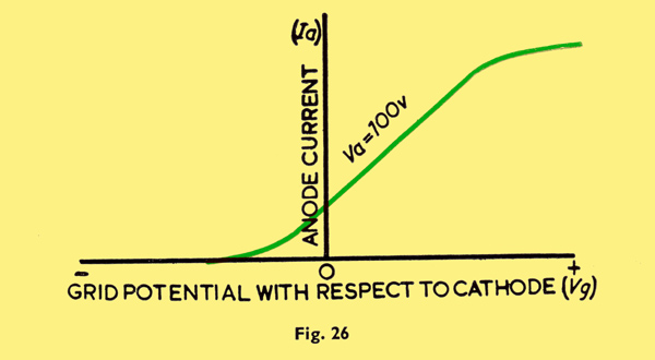
If now a positive potential of, say, 100 Volts is applied to the Anode and a series of potentials, both negative and positive, are applied to the Grid, a corresponding series of values of Anode Current will result. Thus, for one value of Anode Potential a graph can be drawn (Fig. 26 above) showing how Anode Current varies with Grid Potential.
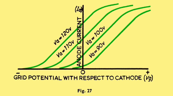
A family of such Characteristic Curves as they are known (Fig. 27) may, therefore, be drawn, each corresponding to a particular Anode Potential.
Obviously since there are three variable quantities-(i) Anode Potential; (ii) Grid Potential; (iii) Anode Current-another family of curves may be drawn (Fig. 28). Each curve now corresponds to a fixed Grid Potential and indicates how Anode Current varies with Anode Potential.
It has been shown that a change in Anode Potential (Va) produces a corresponding change in the Anode Current (la). Generally speaking, it might be expected that this relationship would be uniform and that the graph connecting Va and la would, therefore, be a straight line. Fig. 28, however, shows that this is not altogether the case. Considering the characteristic curve taken at zero Grid Potential it is obvious that over its greater part it is a straight line, but how can we account for the curvature at either end?
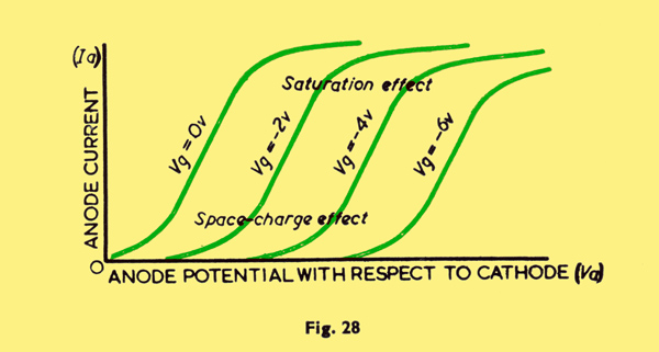
Obviously, when there is no positive potential on the Anode (Va=0), electrons from the Cathode will not be attracted there, hence there is zero Anode Current. In other words, the electrons being emitted from the Cathode, having no urge to go towards the Anode, once their initial impetus has been used up, will merely fall back to the Cathode.
This means that the Cathode will, all this time, be surrounded by a cloud of electrons, the sum of whose individual negative charges will produce a resultant negative charge in the space around the Cathode. It is, in fact, known as the Space Charge.
Since the Anode is, by comparison, so much farther away from the Cathode than is this Space Charge, a small Anode Potential will have very little pull on the emitted electrons. Hence the effect of the Space Charge has to be overcome by having a relatively high Anode Potential before electrons can leap across to the Anode. Once this position has been reached a straight line characteristic ensues, an increase in Anode Potential resulting in a directly corresponding increase in Anode Current.
If now a negative potential is applied to the Grid the Anode Potential will have to be higher still to overcome the combined effect of the Space and Grid Charges. This is reflected in the curves since for increasingly negative Grid Potentials increasingly higher Anode Potentials are needed before Anode Current starts to flow.
At the top end of each characteristic the straight portion bends over until it is running horizontally, indicating that no matter how much more positive the Anode Potential is made there will be no further increase in Anode Current.
When this stage is reached it means, substantially, that all the electrons which the Cathode is capable of emitting are now being drawn to the Anode. The Anode Current has reached Saturation.
If a potential (V) is applied across a conductor and the current (I) is measured, it is found, under normal circumstances, that the ratio Potential (V in Volts) / Current (I in amperes) has a constant value. This value is known as the Resistance of that conductor and it is measured in OHMS.
In fact the relationship (Volts) / (Amperes) = Ohms (or V/I = R) constitutes what is known as Ohm's Law.
Similarly we find that a small change in the applied potential (δV) will produce a small change in the current (δI) and, in addition, that the ratio (δV) / (δI) has the same constant value as the original V/I, that is, R Ohms.
Since the Triode valve itself can act as a conductor it may be considered in the same way, but one glance at anyone of the Ia-V graphs (Fig. 28) will show that the relationship between the applied potential (Va) and the output current (la) cannot have a constant value because of the curvature at the top and bottom of the graph. However, it is in the straight part of the graph that we are most interested.
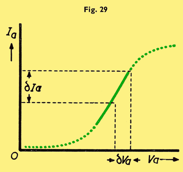
Considering this straight part then (redrawn in Fig. 29) it is plain to see that over this section the relationship between a small change in Anode Potential (δVa) and its consequent small change in Anode Current (δla) will have a constant value. As with the simple conductor, therefore, this relationship (δVa) / (δIa) is measured in Ohms. It is known as the Internal or Anode AC Resistance of the valve and is given the symbol ra. Because we are dealing only with the straight part of the graph it is necessary in a catalogue, by specifying Anode and Grid Potentials, to show to what part of the characteristic curve this resistance applies.
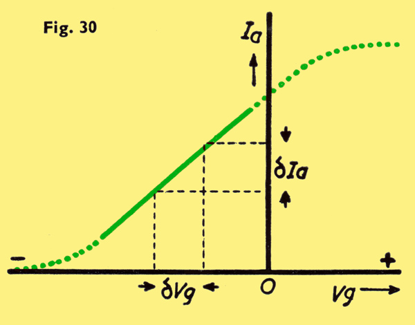
Now the potential applied to the Grid of a Triode is used to control the Anode Current. The degree to which it can do this presents a method of readily assessing the capabilities of the valve. Consequently (see Fig. 30) we want to know what change in Anode Current (δla) there will be for a given change in Grid Potential (δVg) in other words how many milliamps difference in Anode Current there is for a change of one volt in Grid Potential, how many milliamps-per-volt (usually written mA/V).
Now (mA)/(v) is the reciprocal of (V)/(mA) which is one thousandth of V/A (since there are 1,000 milliamperes to one ampere). As we have seen, though, Volts/Amperes gives the value in Ohms, of resistance, But the reciprocal, or opposite, of Resistance (the ability to resist current flow) is, rather obviously, Conductance.(the ability to conduct, or assist current flow). A change in Anode Current (δla) depends on the mutual effect of the change of Grid Potential (δVg). Hence the ratio (δIa)/(δVg) is known as the Mutual Conductance of the valve and is given the symbol gm.
In considering ra the Anode Current (la) and Anode Potential (Va) were variable and the Grid Potential (Vg) was fixed (Fig. 29). To derive gm the Anode Current (la) and Grid Potential (Vg) were variable and the Anode Potential (Va) was fixed. Let us now consider what change in Anode Potential (δVa) is necessary to keep the Anode Current (la) constant if the Grid Potential (Vg) is changed by δVg. For this purpose Fig. 28 has been redrawn as Fig. 31.
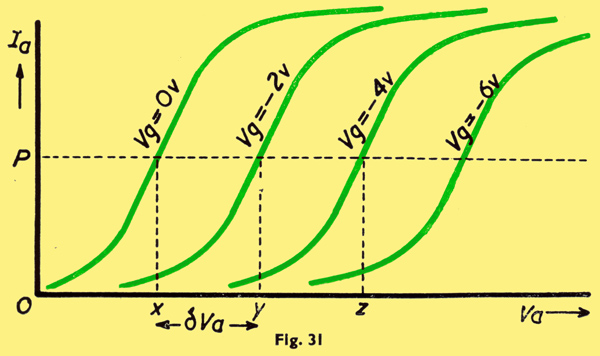
Referring to the Vg=0v characteristic we see that with the Anode Potential at Va=x the Anode Current (la) is P mA. If now we transfer to the V g= -2 v characteristic (that is, in effect, make the Grid Potential more negative) δVg will equal (0 - 2) or -2 Volts and it will be necessary if the Anode Current (la) is to remain at P mA for the Anode Potential (Va) to be increased by δVa to y.
Here, then, we can establish another ratio, this time (δVa)/(δVg) which gives the number of times greater the change of Anode Potential (δVa) is than the change in Grid Potential (δVg) which made it necessary. It is, in fact, the factor by which the valve amplifies the change in Grid Potential and is consequently known as the Grid Voltage Amplification Factor or, more shortly, as the Amplification Factor of the Valve. It is given the symbol μ
These three functions, ra gm and μ are known as the parameters of the valve. Having established that:
ra = (δVa)/(δIa)
gm = (δIa)/(δVg)
μ = (δVa)/(δVg)
it is obvious that by multiplying ra by gm:
ra x gm = (δVa)/(δIa) x (δIa)/(δVg)
therefore ra x gm = (δVa)/(δVg)
But, from the equation for μ above we know that (δVa)/(δVg) = μ
therefore ra x gm = μ
Hence we have a relationship between the parameters so that knowing two of them for one set of conditions the other can readily be found.
We have seen that because the Grid of a Triode is physically nearer to the Cathode than is the Anode a small change in the Grid Potential will cause a much greater change in Anode Current than would a similar change in Anode Potential. Thus a weak audio signal can be fed to the Grid of a Triode and the resultant Anode Current can be sufficiently strong to drive a loudspeaker. The valve, in fact, is acting as an Audio Frequency Amplifier.
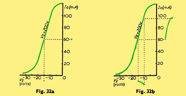
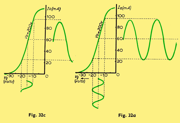
Suppose we take a valve with a characteristic such as that in Fig. 32a. With 200 Volts potential on the Anode and a fixed potential of -15 Volts (bias) on the Grid, it is obvious that the Anode Current will be 60 mA. If on top of this bias of -15 Volts we apply +5 Volts the Grid will then have a potential of ( -15 +5)= -10 Volts. Fig. 32b makes it clear that the Anode Current will increase to 95 mA. Similarly Fig. 32c shows that removal of this applied + 5 Volts and substitution by an additional -5 Volts the Grid will now have a potential of( -15- 5) = -20 Volts. The Anode Current now drops back through 60 mA to 25 mA. In other words, with the valve biased at -15 Volts and with an applied alternating signal (usually termed Grid Swing) of ±5 Volts the Anode Current varies between 95 mA and 25 mA. A change in Grid Potential of from -10 to -20 Volts (10 Volts overall) has produced (95-25) = 70 mA of change in Anode Current.
Now, since that part of the characteristic on which we are working is a straight line, it is clear that whatever the shape of the wave form of the applied alternating signal, the Anode Current, and therefore the output voltage, will have precisely the same wave form (Fig. 32d). This is known as Class A Amplification.
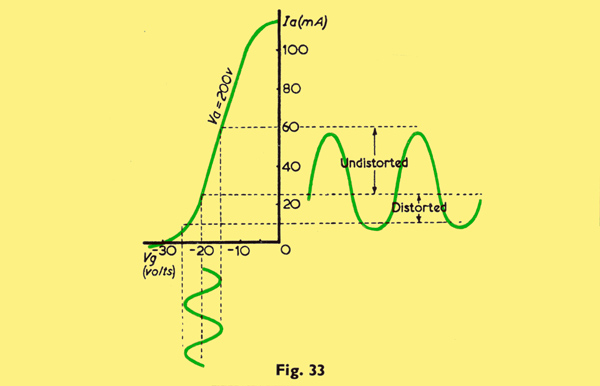
Suppose the valve were wrongly biased at -20 Volts (Fig. 33). Since the Positive Swing (+5 Volts to -15 Volts) is on the straight part of the characteristic it will be reproduced exactly in the Anode circuit. When the Grid Swing is Negative (-5 Volts to -25 Volts) the curved part of the characteristic is in use, and the output wave form will not have the same shape as the input. It will be distorted. If with the Grid biased at -15 Volts a signal were applied of say ±20 Volts it is clear that the Grid Swing would be between -15 +20) = +5 Volts and (-15 -20) = -35 Volts. At those instants of time when the Grid Potential was between 0 Volts and +5 Volts some electrons would be attracted to the Grid instead of to the Anode and Grid Current would flow. This means that the Anode Current would not be true reproduction of the Input Signal, in other words, it would again be distorted.
Now power is measured in Watts and the Watt is a product of Current (I) and Potential (V) or
W = I x V
But from Ohms Law we know that
V = I x R
So, substituting V= I x R in W = I x V we get
W = I x I x R or I²R
But we know, again from Ohms Law, that if we increase R we shall decrease I. So it is obvious that in order to get the greatest possible power output (tat is when i²R has its maximum value) there is one particular or Optimum Value of R.
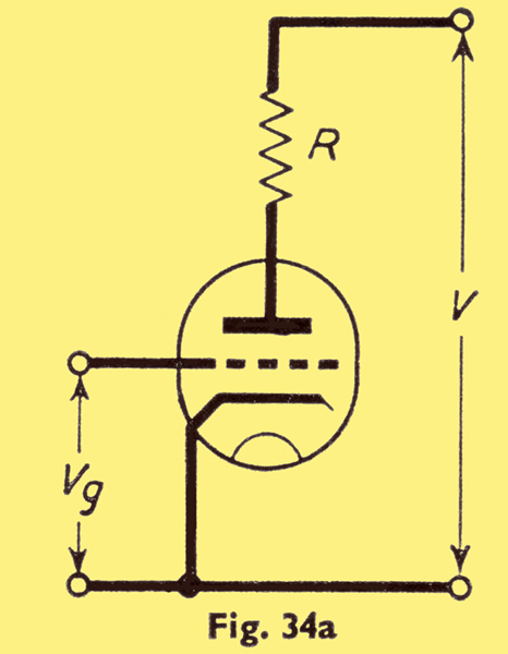
When this argument is applied to the Power Output of a Triode (Fig. 34a) R, for the sake of simplicity, can be considered as the value of the Resistance in the Anode circuit, or, as we say, the Optimum Anode Load. In the specification of a Triode the manufacturer will state what this value should be under certain defined circumstances.
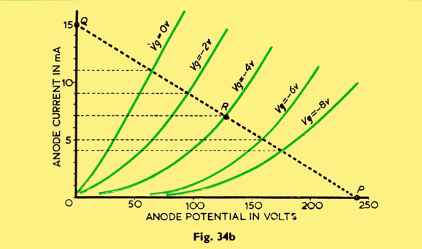
Electrons flowing from Cathode to Anode in Fig. 34a will flow, at the same rate, through the Anode Load, R. If we make the Grid Bias sufficiently negative entirely to cut off Anode Current, the whole of the HT supply voltage will be dropped across the valve. If V= 250 Volts, this state of affairs is represented by point P on Fig. 34b (ie Va = 250V, la = 0 mA). At the other extreme, if the Grid Bias is adjusted so that there is no potential dropped across the valve (ie the valve is acting as a resistance-less conductor) then all the potential (250 Volts) will be dropped across R. So, if we know that the value of R is approximately 16,700 Ohms then again from Ohm's Law.
la = V/R = (250 Volts) / (16,700 Ohms) = 15 mA approx.
So we get Point Q on the curve (ie Va=0v, la = 15 mA). Consequently, by joining points P and Q by a straight line we have what we call the Load Line for this particular value of Anode Load (R).
But what does it tell us? Just this: if the Grid has an initial bias of -4 Volts (point R) there will be a quiescent Anode Current of 7 mA. But if we swing the Grid ±2 Volts (ie between -2 and -6 Volts) the Anode Current will vary between 9 and 5 mA. Further, a change of Grid Voltage from -4 to -2 gives the same change in Anode Current (9 - 7=2 mA) as a change in Grid Voltage from -4 to -6 (7-5=2 mA). Hence the wave form of such a signal fed to the Grid will be reproduced exactly in the Anode circuit and so will be free of distortion.
If, on the other hand, we swing the grid ±4 Volts (ie between 0 and -8 Volts) the change from Vg= -4 to Vg=0 will produce a change in Anode Current of 11 - 7=4 mA, but from Vg= -4 to Vg= -8 gives an Anode Current change of 7 - 4=3 mA. In other words, we shall get distortion of the waveform of the signal fed to the grid since alternate halves will not be similarly reproduced. The Load Line, then, tells us how much we can put in and what we can expect of the valve before there is any distortion.
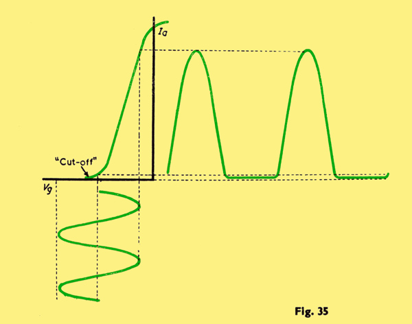
Now consider (Fig. 35) the case of a Triode the Grid of which is biased at cut-off, so that whilst Positive Grid Swings will be amplified due to the straight part of the characteristic, Negative Grid Swings are entirely suppressed. This is known as Class B Amplification.
Unfortunately, owing to the suppression of each half wave, severe distortion results, so, as it stands, this system is no use for Audio Frequency work.
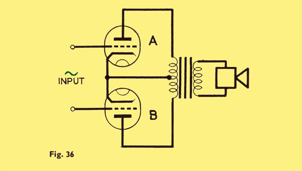
Suppose we connect two of these Class B Amplifiers as shown in Fig. 36. The same alternating input is fed to the two Grids so that when the Grid of Valve A receives a positive pulse, that of Valve B will be negative. Anode Current will then flow in Valve A but it will be suppressed in Valve B. Current thus flowing in the upper half of the primary of the LF Transformer will drive the loudspeaker. The next pulse, however, will be negative to A but positive to B. Hence Anode Current will flow in Valve B but be suppressed in Valve A. Current now flows in the lower half of the primary of the LF Transformer and the loudspeaker will again respond.
Providing the two valves have, as nearly as possible, exactly the same characteristics as each other, or, as we say, are a Matched Pair, each will reproduce an exactly comparable version of those parts of the common input signal which the other suppresses. Thus the severe distortion in a single Class B Amplifier caused by the suppression of alternate signal pulses is overcome in what is known as Class B Push-Pull Amplifier.
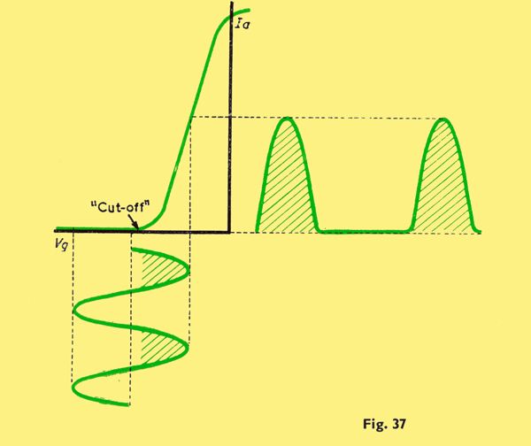
With a valve biased well below cut-off Anode Current will flow during only a small part of each positive pulse of the input signal (shaded in Fig. 37). Consequently, the wave-form of the output signal will be a very distorted version of the input signal, so a Class C Amplifier, as this is called, is no use at all for Audio Frequency Amplification.
The only real relationship the output signal will have with the signal fed to the Grid is that whenever there is a positive pulse in the input there will be a short, badly distorted pulse in the Anode circuit. In other words, the input and output pulses will occur just as often as each other, that is, they will have the same Frequency. Due, however, to this distortion the output will contain many multiples, or Harmonics of this original frequency but, subsequently, if the input signal is of a very High (or Radio) Frequency, we can very easily get rid of them. A Class C Amplifier can, therefore, be used as a Radio Frequency Amplifier.
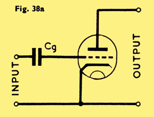
In a Triode the Grid can form an auxiliary Anode so that when a positive potential is applied to it a current-known as Grid Current-- flows between Cathode and Grid. Due, however, to the minute area of this Anode the Grid Current is in the order of micro-amps (millionths) whilst the Anode Current proper is in milliamps (thousandths). Initially, the Grid of the Triode in Fig. 38a is at zero potential (Fig. 38b). When a High Frequency signal is applied to the Grid the first positive half-cycle causes electrons to flow from Cathode to Grid. Consequently, if a capacitor Cg be placed in the Grid lead, a negative charge will be accumulated on it. During the negative half-cycle no Grid Current flows, but as there is no means of discharging Cg it retains its negative charge thus, in effect, biasing the Grid negatively to B - which causes the Anode Current to drop to Q.
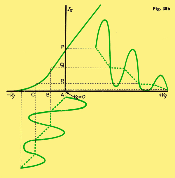
Similarly, the next positive half-cycle further charges Cg and biases the Grid to C. Another drop in Anode Current (to R) ensues and so on until the charge on Cg is sufficient to prevent any flow of Grid Current and hence any further variations of Anode Current. Hence it is necessary to discharge Cg between each successive wave train.
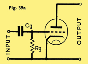
This is accomplished by introducing a Grid Leak, a resistance Rg connected between Cathode and Grid (Fig. 39a). Providing Rg is of sufficiently high a value (in the order of a few megohms-millions of Ohms) the negative charge will still be built up on Cg, but it will discharge during the intervals between each successive wave train thus allowing the Anode Current to return to normal (Fig. 39b).
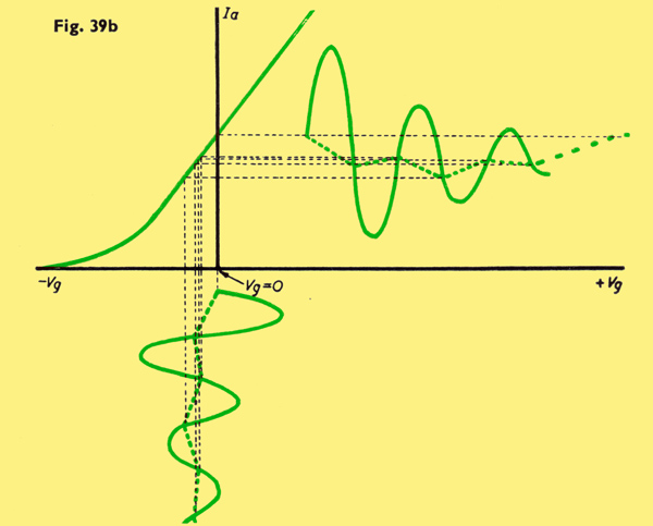
Consequently, if there are 300 wave trains per second, the Anode Current is decreased and allowed to return to normal 300 times per second, so producing an Anode Current variation 300 times per second. But this is an audio frequency, so if telephones are connected across the output terminals an audible 300 Hz note will be heard in them. This is Grid Current Rectification.
If, as was the case in Fig. 35, a Triode is biased at or near cut-off, it is obvious, from what has been said before, that when an alternating signal is fed to the Grid, the positive half-cycles of that signal will permit Anode Current to flow, whilst its negative half-cycles will suppress it. In other words the signal will be rectified or detected.
Thus, if the modulated radio signal of Fig. 8 (in the Diode booklet) is fed to the Grid, the Anode Current will consist of a series of rapid one-way pulses (Fig. 9) the mean value of which can be used, after suitable amplification, to drive a loudspeaker (Fig. 10). The Triode, then, can also be used as a detector of Radio Signals.
In view of the fact that the valve is actually biased to the bend of the Anode Current/Grid Voltage curve, this system is known as Anode Bend Rectification (or Anode-Bend Detection).
A valve designed to fulfil this function is not necessarily required to give amplification of the input signal as was the case with a Class B Amplifier. If amplification were required it would obviously not be practicable to use two valves in push-pull, since that would merely put back the negative pulses we had just taken the trouble to eliminate.
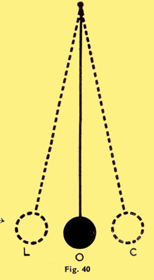
The normal position of the pendulum in Fig. 40 is 0. If it is raised to L it will be given potential energy so that if it is then freed it will swing back to 0 where the energy will become kinetic and cause it to over-swing to C. Here the energy will again become potential so that the pendulum will now swing back again towards L. Due to whatever friction and air resistance there may be the pendulum will not, however, quite reach L, with the result that the potential energy is now very slightly less than it was originally. Consequently, if left to swing backwards and forwards (or, as we say, to oscillate) at its natural frequency the amplitude of the swings would get less and less until eventually the pendulum would once again be motionless in position 0.
In order to keep the pendulum swinging, however, all that would be necessary would be for the minute amount of energy lost in each swing to be replaced at the end of each swing. This, obviously could be done if precisely at the moment the bob reached the end of its swing towards L it were given a little knock in the direction of C. In this way oscillation would be maintained.
It so happens that there is an exact electrical parallel in what is known as the Tuned Circuit.
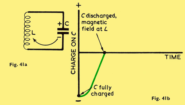
If an electrical potential is applied across a capacitor, the capacitor will become charged. Upon removing the original charging potential the capacitor will retain its potential charge so that if an inductance L be connected across such a capacitor C, charged as shown in Fig. 41a, the surplus of electrons in the lower plate win travel L through L to the positive plate of the capacitor.
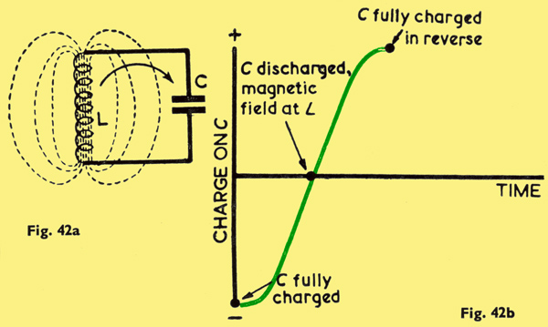
This motion of electrons along the turns of the inductance will cause a magnetic field to be built up within and around it. Once the capacitor is fully discharged (as represented in Fig. 4lb) the magnetic field around L (Fig. 42a) will begin to collapse and in so doing will cause electrons to flow through L and in the same direction. Thus capacitor C again becomes charged, but this time with the upper plate negative and the lower plate positive.
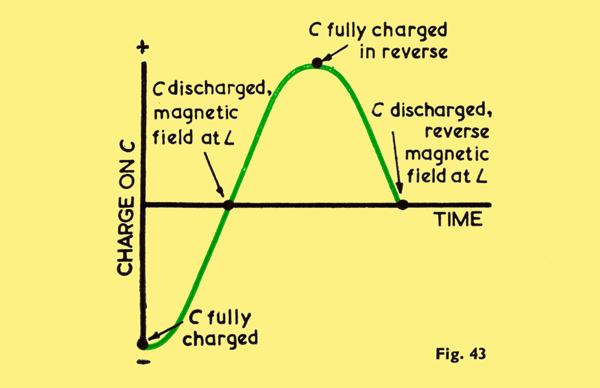
Once the magnetic field has completely collapsed and C is again fully charged (Fig. 42b) C will begin to discharge (Fig. 43), electrons flowing from the upper (negative) plate, through L to the lower (positive) plate, so that a reverse magnetic field is set up around L. Then this field will collapse and so charge up C as shown in Fig. 44.
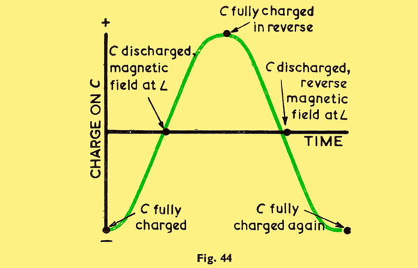
Obviously, then, we are back where we started and the whole cycle of events can be repeated, apparently, ad infinitum. The actual duration of one of these cycles depends directly on the values of L and C; in fact, the number of such cycles, per second, is known as the Natural Frequency of the tuned circuit. Due, however, to resistance losses inherent in the circuit, each successive charge on C will be slightly less than its predecessor. Consequently, if we want to maintain these oscillations, the lost energy must, as in the case of the pendulum, be replaced. This is where the Triode comes in.
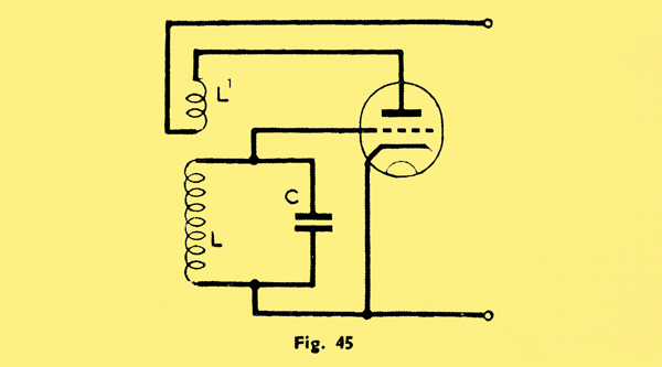
In Fig. 45 the L/C circuit is connected between Grid and Cathode of a Triode. Obviously, the varying potential across C will cause the Anode Current to vary in sympathy. Thus, if a second inductance L¹ is included in the Anode Circuit and it is placed physically near to L the magnetic field round L¹, due to electrons flowing in the Anode circuit, can be made to add itself to that around L. Thus, by careful adjustment of the Coupling between L and L¹ just the right amount of energy can be fed back into the tuned circuit in order that oscillations in it may be maintained. The valve is said to be acting as a Generator of Oscillations or, more colloquially, as an Oscillator;
This is the fundamental principle on which all valve oscillators are founded, though there are many variations, such as the Colpitt's and Hartley circuits.
|