|
This article explains the more obscure causes of difficulties encountered in receiving ultra-short wavelengths, and shows why valves of the Acorn type become increasingly desirable as frequency rises.
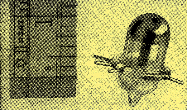
An Acorn valve; specially designed for ultra-high-frequency work.
It is well known to ultra-short-wave experimenters that as the wavelength is reduced far into the single-figure region it becomes almost impossible to obtain any effective amplification by straightforward methods. It is also quite difficult to persuade even an oscillator to function, as designers of ultra-shortwave superheterodyne receivers know to their cost.
Some, at least, of the reasons for this condition of affairs are familiar. For example, there is great difficulty in preventing serious back coupling through even the best screened valve. Then dielectric losses increase as the frequency in creases, or wavelength diminishes. At the lower radio frequencies there is no narrow limit to the tuning capacity that may be used, and it is possible to add a considerable amount to the circuit in such a form as to ensure reasonably small losses. The odd stray capacities over which one has less control, and which generally are rather impure, are thereby made to comprise only a small proportion of the total capacity, and their ability to introduce losses is therefore restricted. At the very high frequencies, however, the total capacity is necessarily so small that the greater part is likely to consist of these relatively inefficient 'strays'.
Another consideration is that, owing to the limited amount of inductance that can be employed in a tuned circuit, the ratio of inductance to capacity (L/C) is low, and as r, the radio-frequency resistance, cannot be made very small, it follows that L/rC cannot be made large. This quantity is well known as the 'dynamic resistance', and is relied upon for building up a large amplified voltage. When multiplied by the mutual conductance g of a high-resistance valve, in the anode circuit of which the dynamic resistance R is connected, the stage gain is approximately gR. For example, 100,000 Ω is quite an easily attainable R at ordinary broadcast or intermediate frequencies, and with the moderate g of 1 mA/V, or 0.001 A/V, the stage gain is 0.001 × 100,000, or 100. But if R, together with any parallel paths formed by valves, etc, cannot be made to exceed 1,000 Ω it is obvious that it is impossible to obtain any amplification at all with this particular valve.
The drop from 100,000 to 1,000, which is by no means fanciful, seems to require a good deal of explanation, and the combined effect of the conditions just described fails to account for than a part of it. The most important factor of all is a rather more obscure one, and the remainder of this article is devoted to it.
One reason why the valve is of such immense value at frequencies lower than those now being discussed is that it acts practically instantaneously. Even although a signal applied to the grid may alternate several million times per second, the anode current responds with no perceptible lag. Suppose, for the sake of argument, that it does lag by one-hundredth of an alternation at a frequency of one Mega Hertz (300 metres). It is clear that the electrons must cross the space inside the valve at a very hot pace indeed to do the journey in 0.00000001 of a second! And that is quite a poor performance for a valve. Actually, one is accustomed to considerably smarter work. But even this standard of agility fails to keep perfect step with ultra-high-frequency oscillations. In ordinary receiving valves some lag is noticeable above about 15 MHz.
In what manner is it noticeable? If it were merely a matter of the amplified signal occurring a few thousand-millionths of a second later than the original, it would of some slight theoretical interest. But although it may not be obvious at first as glance it actually has a very serious-practical-influence.
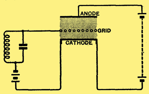
Fig. 1. - Diagram of a triode valve with a uniform distribution of electrons in the space between cathode and anode. When the equilibrium is upset by a very rapid change in grid voltage not only is the total number of electrons changed but, owing to the time required for them to traverse the space, uniformity is momentarily disturbed.
To understand why this is so it is necessary to consider closely what takes place during a single oscillation of a signal in a valve. Fig. 1 shows diagrammatically a simple triode valve. The grid is supplied with a negative bias greater than the peak voltage of the signal, with the object of preventing grid current at any moment during the cycle of oscillation. It is not so negative as to cut off all current to the anode, and this current is indicated by a uniform cloud of dots representing electrons moving from cathode to anode.
Grid Currents
Now, it is well known that when electrons actually land on the grid in greater numbers than those leaving it, this surplus finding its way back to the cathode through the external circuit is what we call a grid current. But it is perhaps not so Well known that, owing to the repulsion of electrical particles of like sign, such a current is set up when the number of electrons approaching the grid exceeds those receding from it, or vice versa.
When a valve is working under the conditions described, with adequate bias, there is, of course, no grid current due to electrons being attracted on to the grid. And at ordinary frequencies the rate at which the grid changes the flow of electrons from cathode to anode is so slow compared with the rate at which the electrons perform this journey that they are never taken by surprise, as it were, so as to lead to a non-uniform distribution in the cathode-anode space.
But when the frequency is very high, this state of affairs does not hold good. To take an extreme example, suppose that the grid potential, which has been such as to permit a steady current to flow across to the anode, is suddenly made so much negative as to cut off all current. A billionth of a second later there are no new electrons coming from the cathode, because the large negative voltage of the grid exerts an overwhelmingly restraining influence. But the space in the valve still contains large quantities of electrons, that were on their way to the anode, but have not yet had time to get there. Those on the anode side of the grid are still moving anode-wards under the attracting influence of the positive voltage there, and are given, as it were, an additional kick in the pants by the sudden disagreeable negative grid voltage. Those on the cathode side of the grid take this same blow in the face, and are driven back on their tracks towards the cathode. In either case electrons are receding from the grid, and none are approaching, so a current flows into the grid by way of the external circuit. The direction of this current is the same as that which the large negative bias would produce if a conducting path were provided between grid and cathode, although no such conductor in the ordinary sense actually exists.
That this is so is evident by reviewing the situation a millionth of a second later. By this time all electrons have been driven from the inter-electrode space; none are moving either towards or away from the grid, and consequently no grid current of any sort is passing. The current that did flow could last only for the minute space of time during which electrons had been surprised into disorderly and irregular ranks.
The process is reversed when a less negative (i.e., relatively positive) potential is suddenly applied to the grid, so that again the current is in the direction that it would take. it a conducting path existed.
If, instead of these isolated instantaneous changes of grid potential, there is substituted an ultra-high-frequency signal, we now have a continuous very rapid change of potential, and the cathode-grid path must be imagined to be there all the time. In practice the resistance of such a path may be quite low - only a few thousands of Ohms - so that it constitutes intolerably heavy damping on any tuned circuit that may be connected. It may, as hinted at the beginning of this article, be so low as to render amplification impossible.
It is therefore important to know what things control the amount of such damping. The subject is very fully dealt with, in theory and practice, by W R Ferris in a paper in the Proceedings of the Institute of Radio Engineers for January, 1936. Some of the controlling factors will be clear from the foregoing account of the phenomenon. The length of the transit time of the electrons is one of them. The transit time, and consequently the grid loss, can be reduced by increasing the anode voltage, so as to accelerate the electrons more rapidly, and by reducing the distance between the electrodes.
These methods are limited by manufacturing difficulties, or by the point at which the gap is broken down by the anode voltage, whichever comes sooner. They have the incidental advantage of increasing the mutual conductance of the valve, and so assisting amplification; but unfortunately this gain is offset by the fact that the mutual conductance happens to be another of the factors controlling grid loss. It is quite easy to see that if the mutual conductance of the valve is large, so that a great body of electrons are controlled by a given change in grid voltage, the undesirable grid current is also relatively large and the equivalent resistance of the valve input is low. Without further information regarding any particular case it is impossible to say whether the net result of enhanced mutual conductance is going to be good or bad.
Losses Increase with Frequency
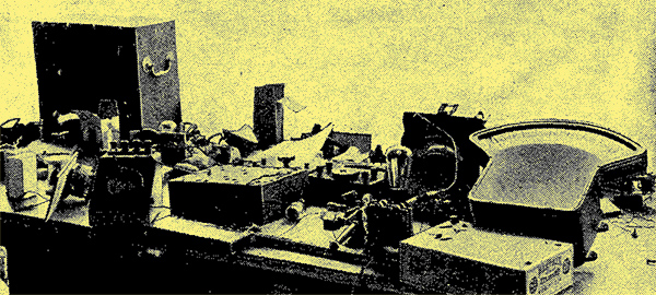
General view of apparatus used for the measurement of grid loss. From right to left are: large scale voltmeter for oscillator bias milliammeter for oscillator anode current; oscillator valve; test circuit; milliammeter for test valve; anode current; test valve battery; battery voltmeter; absorption wave-meter.
Still more obvious is the effect of frequency. The higher the frequency the greater the loss; and the paper by Ferris shows that this factor shares with the transit time the distinction of increasing the loss in proportion to its square. Hence the rapidly increasing difficulty in getting valves to work when the frequency is pushed up into the multi-Mega Hertz.
In addition to these three easily definable factors, the loss is affected to some extent by the dimensions of the valve in ways that cannot be stated in simple form. It is therefore interesting to examine some results of measurements made on typical valves under normal conditions of operation.
The method of measurement at such high frequencies demands careful consideration, when actual circuit quantities differ very widely from those optimistically marked on the diagram. It is a sound principle to make measurements under conditions that resemble as closely as possible those of actual operation. Although one may not then succeed in isolating with theoretical correctness the quantity in question, any divergences therefrom are those that apply in practice.

Fig. 2. - Circuit employed for measuring the grid input resistance of valves at ultra-high frequencies. The left-hand portion represents a valve under test, and the points XX are then made to coincide.
One method is described in Ferris's paper. The present writer has devised an alternative scheme, illustrated in Fig. 2. The right-hand portion represents an oscillating valve with a fixed anode voltage and variable bias. The exact grid voltage at which oscillation can start is measured on a voltmeter with a very extensive scale, and to allow of a wide range of variation a low-impedance type of valve was chosen. It stands in an elevated low-loss holder, and much care was exercised in the placing of the components to reduce connections to a minimum. All tests were made at a frequency of 54 MHz, and as at such frequencies an earth connection of the ordinary type is useless, an artificial earth was made by laying out the circuit above a large copper sheet. Chokes heater or filament currents are, of coarse, of appropriately low resistance. The coil consists of seven turns of No. 16 tinned copper wire ½ in. diameter. As it stands, oscillation starts when the bias is reduced to 11.9 Volts. By connecting various small non-inductive resistors across the oscillatory circuit from the point X to 'earth', other corresponding starting biases are noted, and a curve drawn connecting resistance with grid voltage. By noting the starting bias when an unknown resistance is connected, and referring to the curve, the high-frequency value of the resistance can be determined.
The weak point of this scheme is that one assumes the resistors to maintain their DC values of resistance at such a high frequency. It is known that they do not, and, in evidence of this, resistors of different construction yielded slightly conflicting results. However, the results with the resistors giving the least damping effect were accepted as being the most reliable this agreed with consideration of the resistors themselves - and in any case the probable error is serious only at the high values, which are not of greatest interest for this purpose.
The starting point is detected by a sudden change of anode current, which may be large or small, or a rise or fall. Very smooth control of bias is therefore desirable.
The Testing Circuit
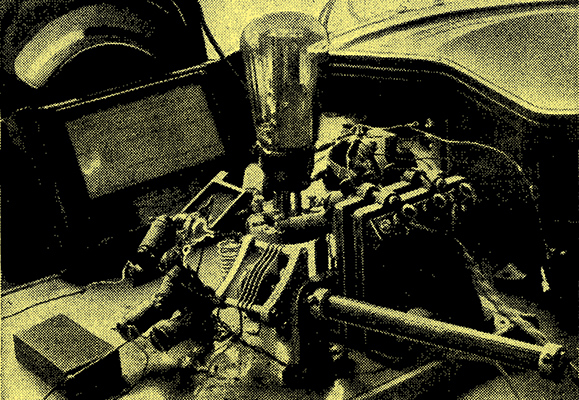
Close-up of test Circuit. Immediately behind the tuning capacitor in the foreground is the oscillator coil, with the oscillator valve to the right and an Acorn valve under test to the left. Note the collection of HF chokes for isolating the test valve from the batteries.
A typical arrangement of a valve at under test is shown to the left of Fig. 2. The separation between XX is merely for the sake of clearness, as, in actual fact it is reduced to an absolute minimum by joining the valve pin direct to the variable capacitor. No valve holder is used, the connections being made with short wires; and the by-pass capacitors lead direct to a single spot close to the earth end of the tuning capacitor. The grid-to-earth path of the valve occupies much the same physical position as did the trial resistors.

For each valve selected for the test the damping is measured first with the valve connected, but cold; secondly with the cathode heated and grid bias applied (to prevent ordinary grid current), but no HT; and thirdly under various full working conditions. The first two results, marked (i) and (ii) in the accompanying table, are generally not greatly different, and they serve to distinguish the sort of loss being studied from those due to other causes. For the reason already mentioned, the figures given in columns (i) and (ii) are of questionable accuracy.
But in each case when anode current is allowed to flow to a normal extent the grid resistance drops to a very low figure. Owing to the method of test, this drop is due solely to the electron lag, and the serious nature of it is thus made apparent. In all these tests the valve is operated with no anode load, as otherwise the effect being studied would be mixed with the 'Miller effect'; and, moreover, the adjustment of anode tuning would be extremely critical.
Although triodes are not generally useful as amplifiers at even low radio frequencies, they are used as oscillators; and the figures given show why oscillation becomes increasingly less free as the frequency is raised. It must be remembered that a resistance of 5,000 Ω at the frequency of test becomes only 1,250 Ω at 108 MHz (just below 3 metres), so that whatever efforts may be made to reduce losses elsewhere are of negligible avail. Another bad effect of the electron lag is that the reaction, on which the maintenance of oscillation depends, comes in the wrong phase to be useful.
The Hivac 'X' valves are midgets, with exceptionally low inter-electrode capacities. This is helpful in reducing the initial loss and in enabling a higher value of inductance to be used, but it does not appear that they confer a very substantial benefit in the shape of reduced lag loss, in relation to mutual conductance. The slightly increased inductance is incidentally helpful in this respect, however, as the grid loss may be reduced by tapping down on the coil.
The second line relating to the XD valve shows how, when the mutual conductance of the valve is lowered, the grid conductance falls too (resistance rises). The XP valve, although of better mutual conductance, inflicts less loss than the XD. The P215 is a full size valve of comparable characteristics.
The Acorn valves are specially designed, by providing very small electrode clearances, to minimise input loss. The success of this construction is strikingly demonstrated by the figures, although the actual values should not be given too much credence as, for reasons explained, they are only very approximate above 25,000 Ω. But it can at least be said that the input resistance of an Acorn under working conditions is higher than that of many valves when 'dead'.
Valves of this type are the only ones capable of direct amplification down to 1 metre and even lower. The mutual conductances are quite high, too, and compare favourably with those of valves of conventional design.
The figures for the AC/VP1 and X41, typical variable-μ pentode and frequency changer respectively, show how heavily the input circuit is damped under the conditions when greatest amplification and selectivity are desired - when signal strength is below the AVC bias starting level.
The desirability of connecting the valve across only a part of the tuned circuit is plain. And again the overwhelming advantage of the Acorn type of construction stands out.
The effect of altering the grid bias, and hence the mutual conductance, is illustrated for several of the types of valves selected. This relationship has been examined in greater detail tor a pair of valves having fairly similar characteristics but different construction - the XP and P215.
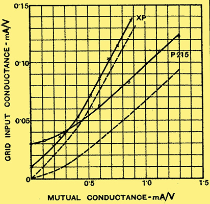
Fig. 3. - Curves showing how the grid input conductance of valves increases almost in proportion to the mutual conductance, but may differ considerably in valves of similar characteristics. The full-line curves show the total conductance, and the dotted curves that due to electron lag only.
Fig. 3 shows curves connecting grid loss with mutual conductance. To make the relationship clearer, the loss also has been expressed as a conductance - the reciprocal of the grid input resistance. For one thing, the electron lag effect can be separated from the other valve losses with the greatest of ease by simply subtracting the conductance under the condition of zero anode current; i.e. , by dropping the curves bodily until they pass through the origin.
It is now possible to see that the miniature valve is not necessarily advantageous for ultra high-frequency work, and may actually cause more than double the electron-lag loss for a given mutual conductance. These curves also support the theory that for a given valve the grid input conductance is proportional to the mutual conductance - at any rate above the bottom bend of the valves characteristic curves.
Diode valves have not yet been mentioned; for ordinary receiver purposes the electron lag is not very important, but for valve voltmeter purposes it certainly is. For a very full investigation of this, refer to E C S Megaw's article in The Wireless Engineer, February, March and April, 1936. It is sufficient to point out that the triode valve voltmeter is not to be recommended at ultra-high frequencies, because of its low input resistance.
|